Disjoint sets are used to solve a problem called dynamic connectivity.
This data structure has two operations:
connect(x, y): connectsxandyisConnected(x, y): returns true ifxandyare connected. Connections don’t need to be direct (transitive)
Note: The ideas and content (including images) in this post come from Josh Hug’s excellent lectures from UC Berkeley’s CS61B.
Introduction
Let’s consider an example. We start with a set of 7 integers from 0 to 6 connected as follows:
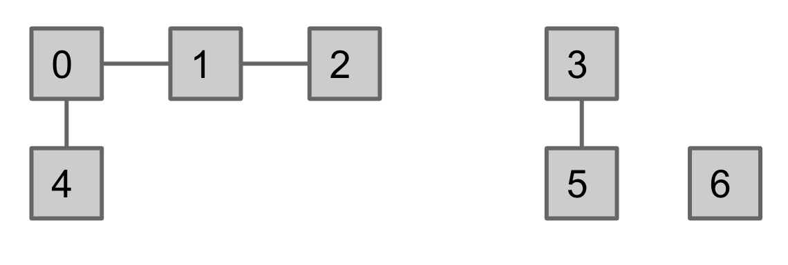
We achieve this by doing something like:
ds = DisjointSets(7)
ds.connect(0, 1)
ds.connect(1, 2)
ds.connect(0, 4)
ds.connect(3, 5)
Next, if we check for connectivity between elements, we should get the following responses:
ds.isConnected(2, 4) // true
ds.isConnected(3, 0) // false
If we then do the following operations, we expect this behaviour:
As seen in the video, in the end, all of the elements will belong to the same set, ie, every element will be connected to every other element.
Seems like a pretty simple problem. But, as we’ll see going forwards, we’re not just concerned with solving it correctly, we want to solve it as fast as we can.
Implementation
Set Membership
Let’s start with a naive approach to solving this problem. We could, using some data structure, keep track of every single line connecting two elements. And then while checking for connectedness, we could perform some form of iteration over these lines to see if one item could be reached from another. However, this is way too complicated an approach to begin with. After pondering a bit on this problem, we can see that we don’t need to keep track of every line between connected components, rather, we just need to keep track of the sets each component belongs to. So, this same operations shown above would result in sets like this:
| operation | sets/output |
|---|---|
| {0}, {1}, {2}, {3}, {4}, {5}, {6} | |
| connect(0, 1) | {0, 1}, {2}, {3}, {4}, {5}, {6} |
| connect(1, 2) | {0, 1, 2}, {3}, {4}, {5}, {6} |
| connect(0, 4) | {0, 1, 2, 4}, {3}, {5}, {6} |
| connect(3, 5) | {0, 1, 2, 4}, {3, 5}, {6} |
| isConnected(2, 4) | true |
| isConnected(3, 0) | false |
| connect(4, 2) | {0, 1, 2, 4}, {3, 5}, {6} |
| connect(4, 6) | {0, 1, 2, 4, 6}, {3, 5} |
| connect(3, 6) | {0, 1, 2, 3, 4, 5, 6} |
| isConnected(3, 0) | true |
This approach makes the problem much easier to solve. In essence, we’re not concerned with HOW the elements are connected, rather, we’re just concerned IF they are connected or not.
Our next concern is to figure out what instance variables to use to keep track of set membership. Again, let’s start with a naive approach to this.
List of Sets
We could store the sets in a list, eg. [{0}, {1}, {2}, {3}, {4}, {5}, {6}]. In Java, we’d use List<Set<Integer>> to do that. However, it’s pretty clear that isConnected would take Θ(N) time in the worst case — where nothing would be connected, and we’d have to iterate over the entire list. The same is true for the constructor of the data structure, and the connect operation. In summary, here are the runtimes.
| Implementation | constructor | connect | isConnected |
|---|---|---|---|
| ListOfSetsDS | Θ(N) | O(N) | O(N) |
Note: When trying to implement a higher level data structure using basic building blocks, the choice of the building blocks will DEEPLY affect the complexity of the code, and its performance.
Quick Find: List of Integers
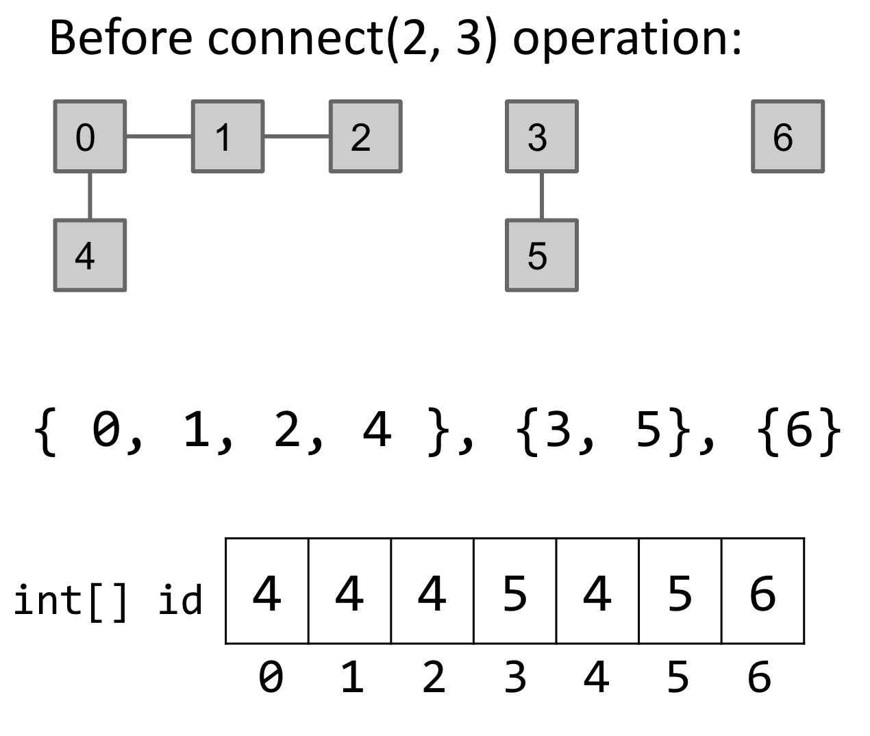
We can improve this data structure by simply representing connected components as a list of integers. Here’s how that would work: Instead of representing { 0, 1, 2, 4 }, {3, 5}, {6} as [{0, 1, 2, 4}, {3, 5}, {6}] — ie a list of sets of integers — we’ll represent them as [4, 4, 4, 5, 4, 5, 6]. Each element will point to a single element from the set of which it is a member of. In this case, 0, 1, 2, and 4 point to 4. Here’s how a connect operation would work with this approach:
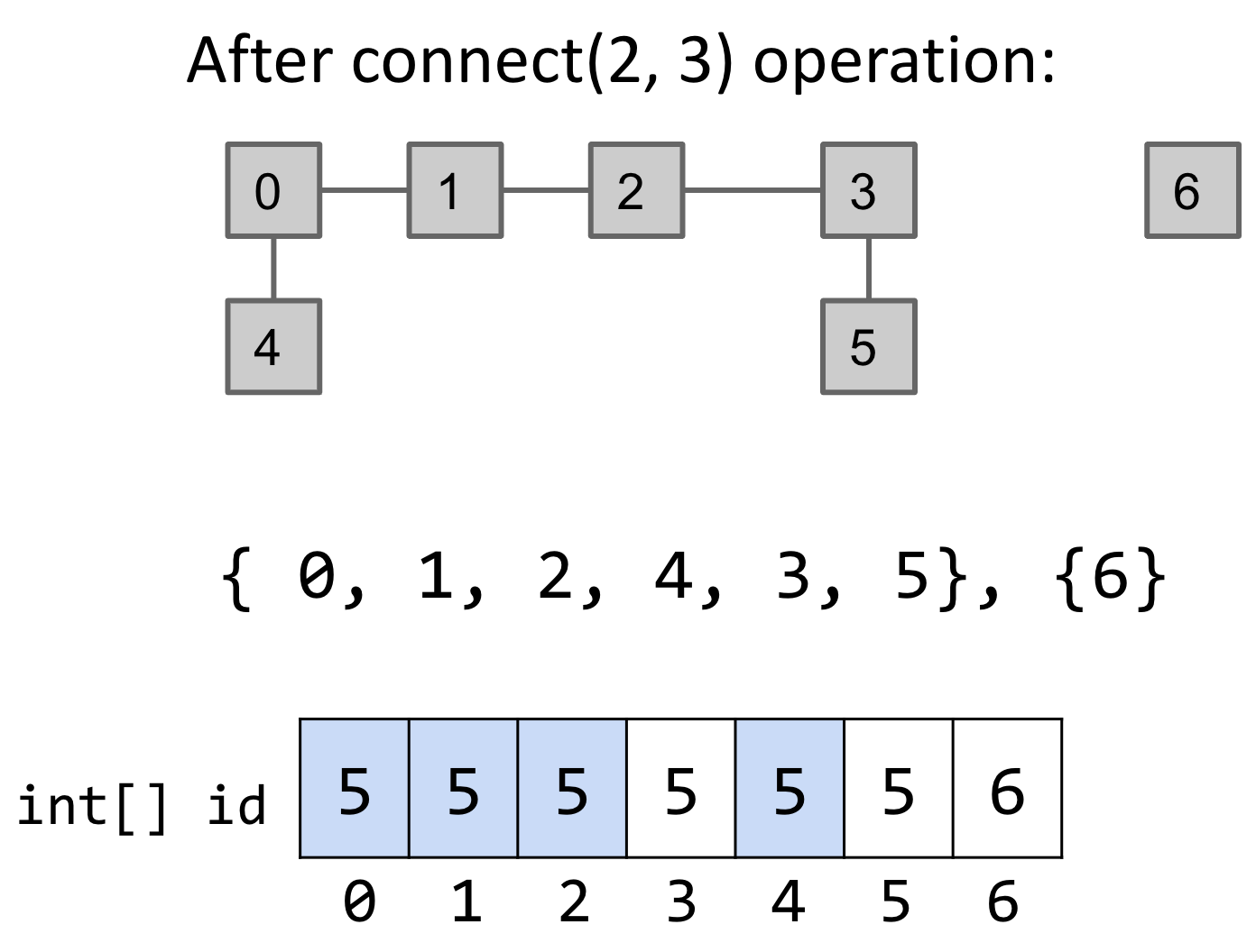
In summary, we make sure that all of the items that point to the element that 2 points to (ie 4) now point to the element that 3 points to (ie 5). A benefit of this approach is that the isConnected operation will Θ(1) since we just need to check if the values at two indices are same or not. However, connect will be Θ(N) as we still have to iterate over the entire list to change values. Here’s the summary of runtime performance of all approaches so far:
| Implementation | constructor | connect | isConnected |
|---|---|---|---|
| ListOfSetsDS | Θ(N) | O(N) | O(N) |
| QuickFindDS | Θ(N) | Θ(N) | Θ(1) |
Quick Union
For the next approach, we will still represent everything as connected components, and represent connected components as a list of integers. However, the values in the list will be chosen so that connect is fast.
As seen before, the slowness of the connect operation comes from having to change multiple values in the list while combining two sets. If we could change our set representation so that combining two sets required only changing one value, that would radically improve the performance of the data structure. Here’s the key idea behind the solution:
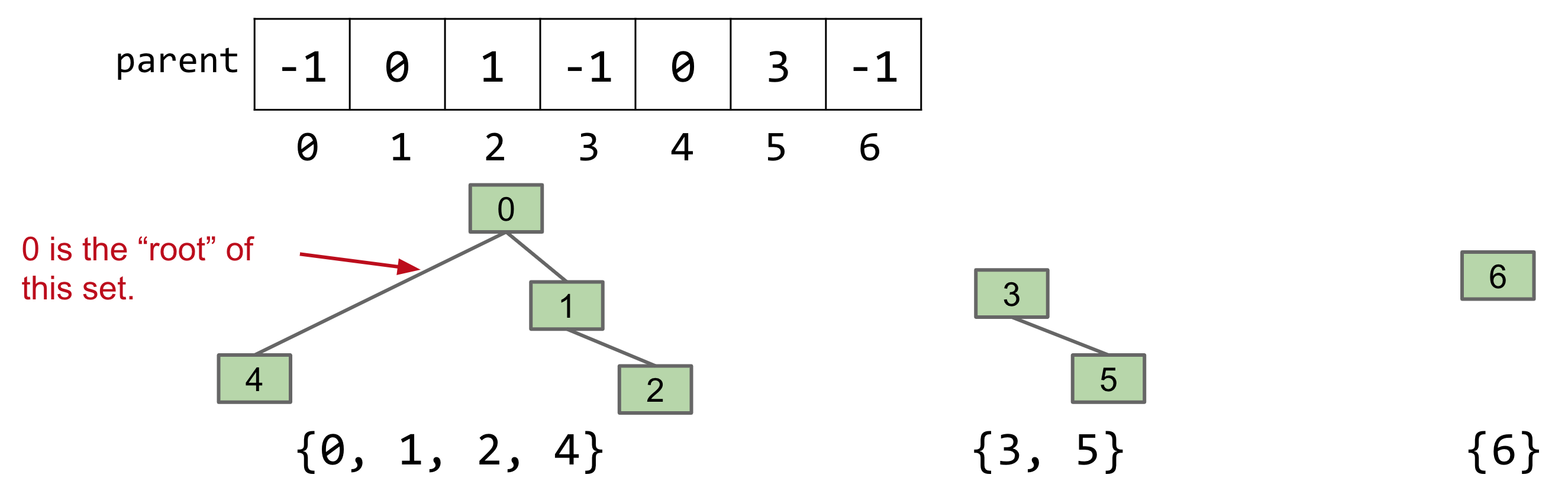
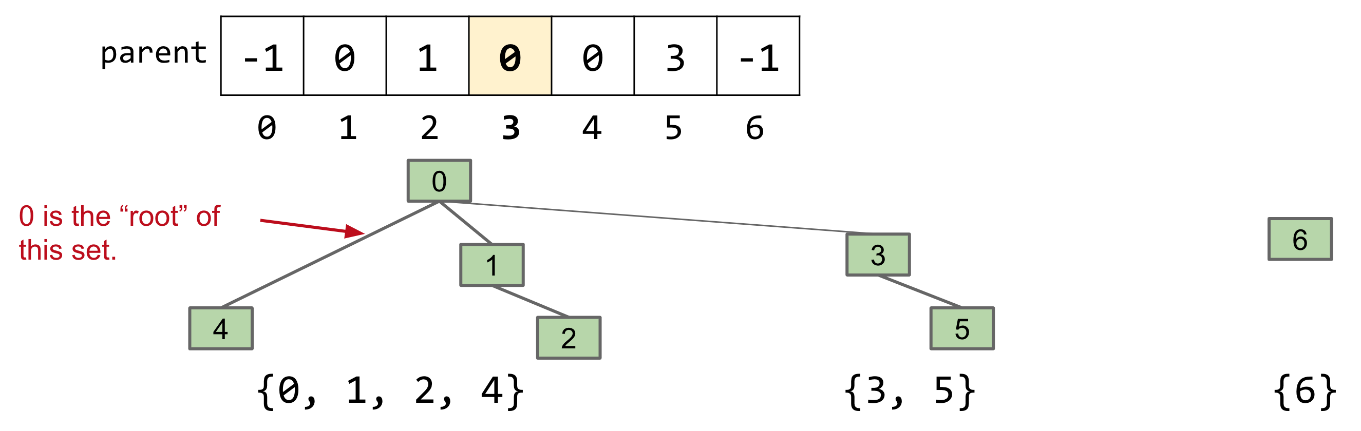
Instead of assigning each item an ID, we’ll assign it a parent. This would result in a tree-like structure.
Using this approach, here’s how the sets shown before would be represented:
Next, let’s see how a connect would look like with this approach. If we need to perform connect(5, 2), we can’t just set the value of 5 to be 2, since that would isolate 3 as a separate group. Instead, we find the roots of both 5 and 2, and set the value of 5’s root to be equal to 2’s root. That would result in the value of 3 being set to 0, as follows:
It might seem that connect entails only changing one value, but finding the roots can be expensive depending on how the trees are constructed — we might end up with a very long imbalanced tree. This would result in Θ(N) performance in the worst case for both connect and isConnected. This idea seems to be a step in the right direction if we could somehow keep the trees balanced, which we’ll solve with the next approach. Here’s the summary of runtime performance of all approaches so far:
| Implementation | Constructor | connect | isConnected |
|---|---|---|---|
| ListOfSetsDS | Θ(N) | O(N) | O(N) |
| QuickFindDS | Θ(N) | Θ(N) | Θ(1) |
| QuickUnionDS | Θ(N) | O(N) | O(N) |
Weighted Quick Union
Weighted Quick Union is a modification of the Quick Union algorithm to avoid tall trees. To understand how it works, let’s consider the connect(2, 5) operation shown below. We could either make 5’s root a child of 2’s root, or the other way around. The former would result in a tree of height 2, while the latter would result in a tree of height 3. Since the worst case performance of the data structure depends on the height of the tree, the former approach is better.
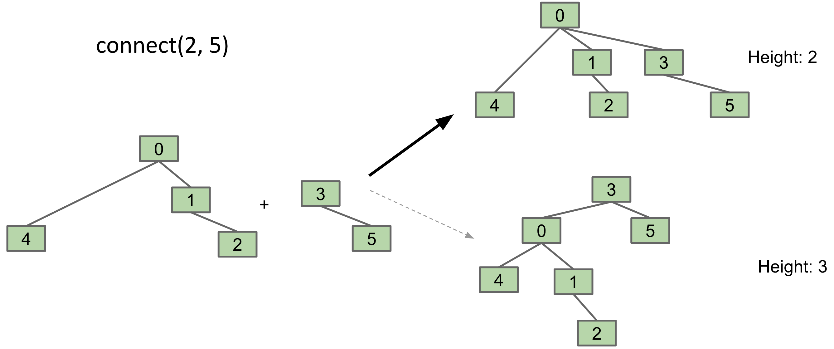
The key idea behind Weighted Quick Union is that we’ll somehow keep track of tree size (ie number of elements), and always link root of smaller tree to root of larger tree.
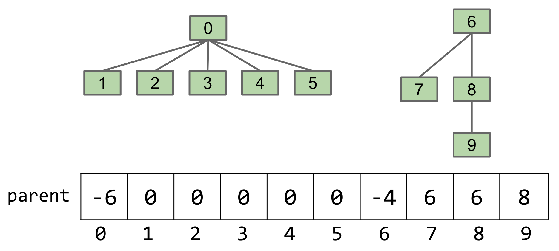
Tree size can be tracked with a minor modification to how the parent array is represented. Instead of just representing the value of a root node as -1, we store it as the negative of the size of its tree. In other words, a root node with a tree size of 6 will have a value of -6 in the parent array. For example, the following shows a specific set membership scenario, and its corresponding parent array.
Next, let’s consider runtime performance of this approach. Since the performance of connect and isConnected depends on the height of the tree H, let’s analyse how fast it grows with respect to the number of elements being tracked N. Due to the fact that we always make a smaller tree a child of the larger one, N needs to double for an increment in the height of the tree. The following video shows the worst case where tree height grows as fast as possible.
This behaviour indicates a logarithmic increase in H with respect to N in the worst case. As a result, the asymptotic runtime of both connect and isConnected is O(logN). Here’s the summary of runtime performance of all approaches so far:
| Implementation | Constructor | connect | isConnected |
|---|---|---|---|
| ListOfSetsDS | Θ(N) | O(N) | O(N) |
| QuickFindDS | Θ(N) | Θ(N) | Θ(1) |
| QuickUnionDS | Θ(N) | O(N) | O(N) |
| WeightedQuickUnionDS | Θ(N) | O(log N) | O(log N) |
Weighted Union with Path Compression
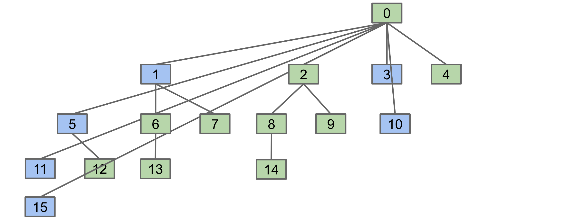
We’ve already achieved logarithmic runtime performance by tweaking the Quick Union algorithm to consider tree sizes whilst connecting items. Now, let’s do even better by making use of a technique called “path compression”. To understand it, let’s consider the following example where we want to perform the operation isConnected(15, 10).
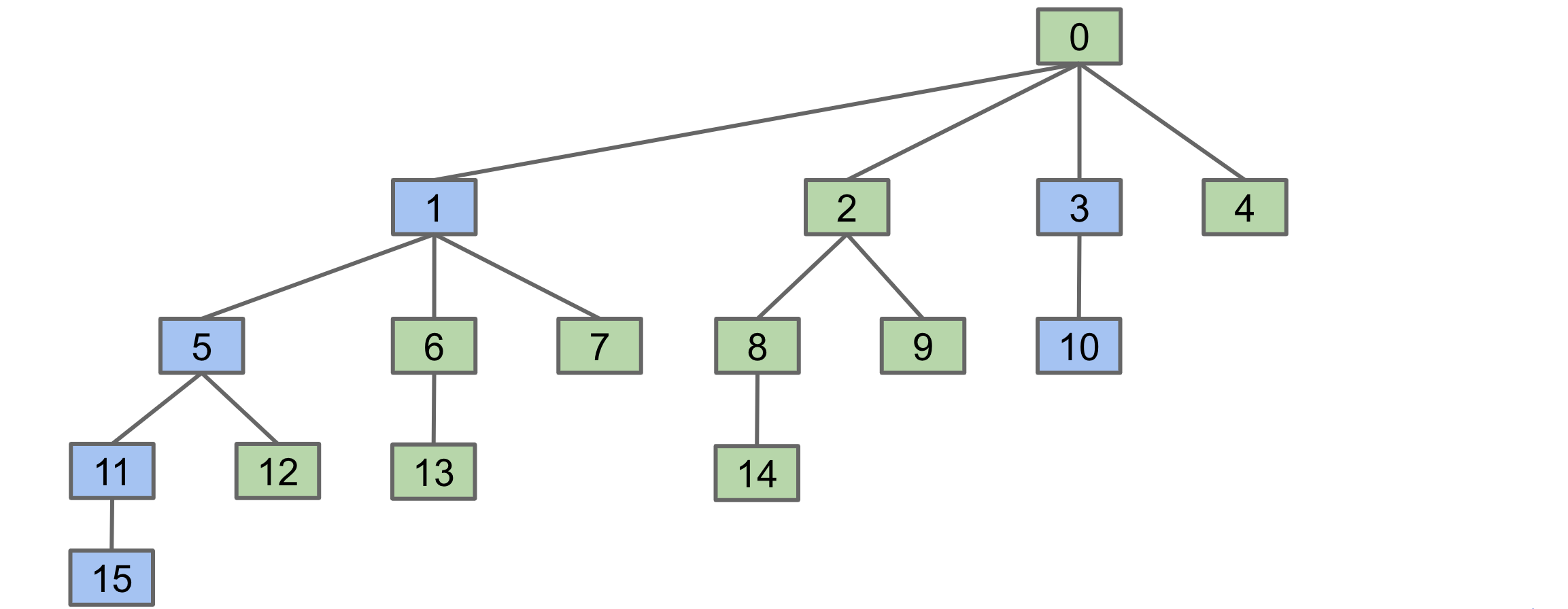
With our approach so far, we’ll climb up the tree starting from 15 till we find the root 0. While doing that, we’ll traverse through nodes 11, 5, and 1. Since we know for a fact that these 3 nodes also belong to the set of which 0 is the root of, we could just set the parent of each of these nodes to be 0. This would shorten the path to be traversed in finding the root of these nodes in subsequent isConnected and connect operations. We’ll do the same for the path from 10 to 0. Finally, we’ll end up with a tree looking like this.
We can rearrange this tree to look like this:
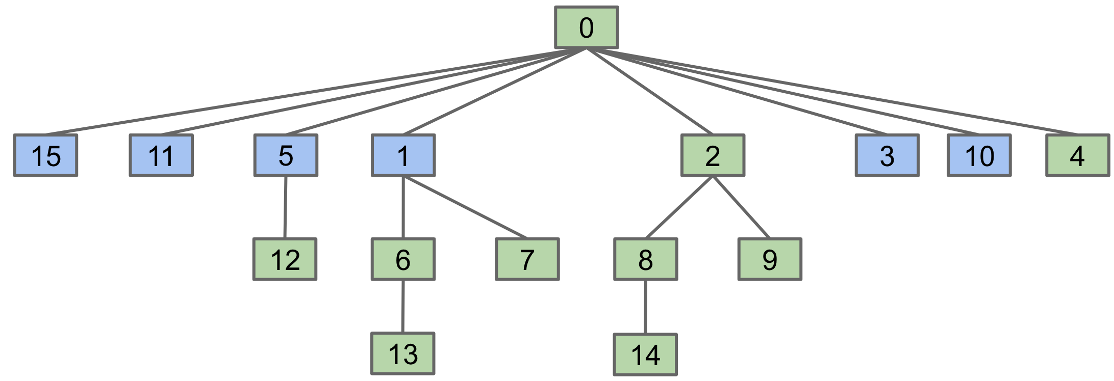
As seen above, the paths from 15, 11, 5, and 10 have shortened to a hop of just 1. The additional cost of doing this is insignificant, ie, it is the same order of growth as before, but subsequent queries will be faster. If we keep compressing paths like this, we’ll make the tree flatter and flatter after each operation.
Here’s how these operations can be implemented. In this implementation, union is what we’re referring to as connect so far, while the actual connect operation is a private helper function for union. connected is what we’re referring to as isConnected, and find is helper function used by connect and connected.
/**
 * The "connect" operation as described in this post.
 */
public void union(int v1, int v2) {
    int size1 = sizeOf(v1);
    int size2 = sizeOf(v2);
    if (size1 > size2) {
        // connect v2 to root of v1's set
        connect(v2, v1);
    } else {
        // connect v2 to root of v2's set
        connect(v1, v2);
    }
}
/**
 * Helper function for union.
 */
private void connect(int v1, int v2) {
    int rootOfLargerTree = find(v2);
    int rootOfSmallerTree = find(v1);
    if (rootOfLargerTree != rootOfSmallerTree) {
        int sizeOfSmallerTree = sizeOf(rootOfSmallerTree);
        sets[rootOfSmallerTree] = rootOfLargerTree;
        sets[rootOfLargerTree] -= sizeOfSmallerTree;
    }
}
/**
 * The "isConnected" operation described in this post.
 */
public boolean connected(int v1, int v2) {
    if (find(v1) == find(v2)) {
        return true;
    }
    return false;
}
/**
 * Returns the root of the set V belongs to. Path-compression is employed
 * allowing for fast search-time.
 */
public int find(int vertex) {
    if (sets[vertex] < 0) {
        //vertex is a root node
        return vertex;
    }

    //immediate parent is root, no need for path compression
    if (sets[sets[vertex]] < 0) {
        return sets[vertex];
    }

    //compress path
    int currentIndex = vertex;
    LinkedList<Integer> chain = new LinkedList<>();
    while (sets[currentIndex] >= 0) {
        chain.add(currentIndex);
        currentIndex = sets[currentIndex];
    }
    // currentIndex is now the root vertex
    ListIterator iterator = chain.listIterator(chain.size());
    while (iterator.hasPrevious()) {
        sets[(int) iterator.previous()] = currentIndex;
    }
    return currentIndex;
}
The entire implementation code can be found here.
Summary
Let’s revisit the ideas that made our implementation efficient:
- Represent sets as connected components (don’t track individual connections).
- List of Sets: Store connected components as a List of Sets (slow, complicated).
- Quick Find: Store connected components as set ids.
- Quick Union: Store connected components as parent ids.
- Weighted Quick Union: Also track the size of each set, and use size to decide on new tree root.
- Weighted Quick Union With Path Compression: On calls to connect and isConnected, set parent id to the root for all items seen.
References
- Josh Hug’s lectures from CS61B.