I’m quite interested in understanding and interpreting how convnets “see” and process input images that we feed them. I first got a taste of this kind of work after reading Visualizing and Understanding Convolutional Networks by Matthew D Zeiler and Rob Fergus, which is 5 years old as of today. I’m guessing a lot of work has been/is being done by the deep learning research community to make convnets more intuitive and understandable. I’m trying to take strides towards understanding that work.
This post/notebook is an exercise in generating localization heat maps to help visualise areas of an image which contribute the most when making a prediction. Inspiration for this comes from a fastai Deep Learning MOOC (2018) lecture which is itself inspired by Grad-CAM: Visual Explanations from Deep Networks via Gradient-based Localization by Ramprasaath R. Selvaraju, Michael Cogswell, Abhishek Das, Ramakrishna Vedantam, Devi Parikh, Dhruv Batra.
Setup
I’m using The Oxford-IIIT Pet Dataset for this experiment, which is hosted for fastai by AWS here.
%reload_ext autoreload
%autoreload 2
%matplotlib inline

from fastai import *
from fastai.vision import *
bs = 32 #batch size
path = untar_data(URLs.PETS)/'images'
Data Augmentation
Setting up a data generator which also augments the data based on various transforms. More on fastai’s transforms here.
tfms = get_transforms(max_rotate=20, max_zoom=1.3, max_lighting=0.4, max_warp=0.4,
                      p_affine=.2, p_lighting=.2)
src = ImageItemList.from_folder(path).random_split_by_pct(0.2, seed=2)
def get_data(size, bs, padding_mode='reflection'):
    return (src.label_from_re(r'([^/]+)_\d+.jpg$')
           .transform(tfms, size=size, padding_mode=padding_mode)
           .databunch(bs=bs).normalize(imagenet_stats))
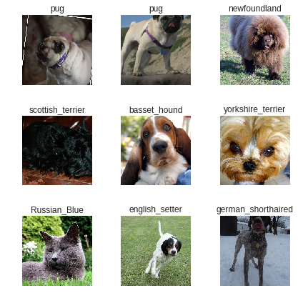
data = get_data(224, bs)
data.show_batch(rows=3, figsize=(6,6))
Training
I’ll be using ResNet-34’s architecture for this network. Fastai’s create_cnn handles altering the final fully connected layer to output a 37 dimensional output behind the scenes. This is done based on the number of classes in the dataset which is stored as data.c. The classes themselves are stored in data.classes.
print(data.c)
37
print(data.classes)
['Abyssinian', 'Bengal', 'Birman', 'Bombay', 'British_Shorthair', 'Egyptian_Mau', 'Maine_Coon', 'Persian', 'Ragdoll', 'Russian_Blue', 'Siamese', 'Sphynx', 'american_bulldog', 'american_pit_bull_terrier', 'basset_hound', 'beagle', 'boxer', 'chihuahua', 'english_cocker_spaniel', 'english_setter', 'german_shorthaired', 'great_pyrenees', 'havanese', 'japanese_chin', 'keeshond', 'leonberger', 'miniature_pinscher', 'newfoundland', 'pomeranian', 'pug', 'saint_bernard', 'samoyed', 'scottish_terrier', 'shiba_inu', 'staffordshire_bull_terrier', 'wheaten_terrier', 'yorkshire_terrier']
gc.collect()
learn = create_cnn(data, models.resnet34, metrics=error_rate, bn_final=True)
Downloading: "https://download.pytorch.org/models/resnet34-333f7ec4.pth" to /root/.torch/models/resnet34-333f7ec4.pth
100%|██████████| 87306240/87306240 [00:01<00:00, 83351997.05it/s]
learn.fit_one_cycle(3, slice(1e-2), pct_start=0.8)
Total time: 04:55
epoch	train_loss	valid_loss	error_rate
1	2.148532	1.041757	0.173207
2	1.111558	0.338378	0.102165
3	0.740522	0.288959	0.077131
learn.unfreeze()
learn.fit_one_cycle(2, max_lr=slice(1e-6,1e-3), pct_start=0.8)
Total time: 03:30
epoch	train_loss	valid_loss	error_rate
1	0.705978	0.266104	0.067659
2	0.620636	0.266208	0.071719
data = get_data(352,bs)
learn.data = data
learn.fit_one_cycle(2, max_lr=slice(1e-6,1e-4))
Total time: 03:30
epoch	train_loss	valid_loss	error_rate
1	0.705978	0.266104	0.067659
2	0.620636	0.266208	0.071719
learn.save('352')
The model predicts 37 classes of dogs and cats with a 5.0744% error rate on the validation dataset. That’s good enough for this experiment.
Non class-discriminative heat-maps
One of the reasons why convolutional layers are used for deep learning on image data is that they naturally retain spatial information present in the inputs which is manipulated to represent high-level semantics as we move deeper in the network, and is finally handed over to fully connected layers that come up with the relevant outputs based on their weights and biases.
Selvaraju et al. state in their paper:
we can expect the last convolutional layers to have the best compromise between high-level semantics and detailed spatial information. The neurons in these layers look for semantic class-specific information in the image (say object parts).
Activations of these feature maps can be directly used to visualise which parts of an image the network “focuses” on the most. This might not be instinctively apparent at first (it surely wasn’t for me), but it works. Let’s see that in action.
data = get_data(352,16)
learn = create_cnn(data, models.resnet34, metrics=error_rate, bn_final=True).load('352')
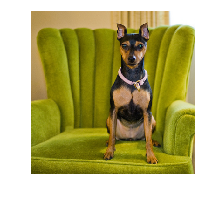
Let’s work with this image of a miniature_pinscher.
idx=4
x,y = data.valid_ds[idx]
x.show()
print(f'class name: {y}\nclass_index: {y.data}')
class name: miniature_pinscher
class_index: 26
Fastai’s learn.model for a CNN is of type torch.nn.modules.container.Sequential of length 2. The first element of this model is another torch.nn.modules.container.Sequential which contains all of the convolutional layers, while the second element contains the fully connected layers.
type(learn.model)
torch.nn.modules.container.Sequential
len(learn.model)
2
In order to get the activations of the feature maps of the last convolutional layer, we need to place a Hook on the output of this layer.
from fastai.callbacks.hooks import *
m = learn.model.eval();
xb,_ = data.one_item(x)    #get tensor from Image x
xb_im = Image(data.denorm(xb)[0])
xb = xb.cuda()
def non_class_discriminative_activations(xb):
    with hook_output(m[0]) as hook_a:
        preds = m(xb)
    return hook_a
hook_a = non_class_discriminative_activations(xb)
acts  = hook_a.stored[0].cpu()
acts.shape
torch.Size([512, 11, 11])
As expected, the shape of the activations of the final convolutional layers is (512,11,11), where 512 is the number of channels, and 11 is both the height and width of the feature maps.
Now let’s do something that felt totally unintuitive to me the first time I did it. Let’s average the values of these activations over the channel axis to get a (11,11) tensor.
avg_acts = acts.mean(0)
avg_acts.shape
torch.Size([11, 11])
We have an (11,11) tensor that represents the spatial information captured by the convnet till the last convolutional layer averaged over the channels axis. Let’s plot it in 2 dimensions.
plt.imshow(avg_acts, cmap='magma');
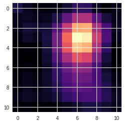
This definitely looks to be concentrated at the face of the miniature_pinscher image above. Let’s plot the input image with the heatmap over it. The (11,11) tensor can be extrapolated to the size of the input, ie (352,352), by using the extent argument of imshow.
def show_non_class_discriminative_heatmap(x):
    xb,_ = data.one_item(x)
    xb_im = Image(data.denorm(xb)[0])
    xb = xb.cuda()
    hook_a = non_class_discriminative_activations(xb)
    acts  = hook_a.stored[0].cpu()
    avg_acts = acts.mean(0)

    _,ax = plt.subplots()
    xb_im.show(ax)
    ax.imshow(avg_acts, alpha=0.6, extent=(0,352,352,0),
              interpolation='bilinear', cmap='magma');
show_non_class_discriminative_heatmap(x)
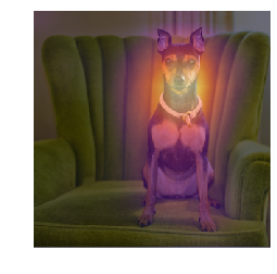
It actually works!! Let’s do this for a bunch of images.
import random
def plot_non_class_disc_multi():
    random.seed(25)

    val_size = len(data.valid_ds)

    fig,ax = plt.subplots(2,4)
    fig.set_size_inches(12,6)

    for i in range(2):
        for j in range(0,4,2):
            idx=random.randint(0, val_size)
            x,y = data.valid_ds[idx]
            xb,_ = data.one_item(x)
            xb_im = Image(data.denorm(xb)[0])
            xb = xb.cuda()
            hook_a = non_class_discriminative_activations(xb)
            acts  = hook_a.stored[0].cpu()
            avg_acts = acts.mean(0)
            xb_im.show(ax[i,j])
            xb_im.show(ax[i,j+1])
            ax[i,j+1].imshow(avg_acts, alpha=0.6, extent=(0,352,352,0),
                      interpolation='bilinear', cmap='magma');
    plt.show()
plot_non_class_disc_multi()
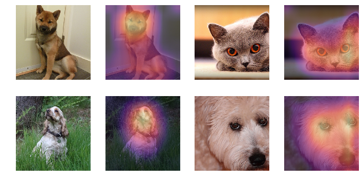
So it’s pretty clear that a properly trained convnet does retain spatial information till the convolutional layers in such a way that the values of the activations of the feature maps correspond to the position of pixels that play a part in coming up with a prediction.
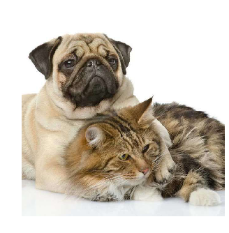
Let’s generate the heat-map for an image that contains objects belonging to two classes
!wget https://i.pinimg.com/originals/ae/e4/a7/aee4a7df36c2e17f2490036d84f05d1f.jpg -O pug_maine.jpg
--2018-12-02 13:15:55--  https://i.pinimg.com/originals/ae/e4/a7/aee4a7df36c2e17f2490036d84f05d1f.jpg
Resolving i.pinimg.com (i.pinimg.com)... 23.35.16.55, 2600:1418:3:29a::1931, 2600:1418:3:298::1931
Connecting to i.pinimg.com (i.pinimg.com)|23.35.16.55|:443... connected.
HTTP request sent, awaiting response... 200 OK
Length: 50986 (50K) [image/jpeg]
Saving to: ‘pug_maine.jpg’

pug_maine.jpg       100%[===================>]  49.79K  --.-KB/s    in 0.01s

2018-12-02 13:15:56 (3.68 MB/s) - ‘pug_maine.jpg’ saved [50986/50986]
fn = 'pug_maine.jpg'
x_test = open_image(fn)
x_test.size
torch.Size([679, 660])
x_test.show(figsize=(x_test.size[0]/120,x_test.size[1]/120))
Let’s see what class does the model predict for this image.
learn.predict(x_test)[0]
Category pug
It classifies the image as pug. The model is trained on single-class data, so that’s fair enough. Let’s check out the heat map for this image.
show_non_class_discriminative_heatmap(x_test)

Hmm. Since the model classified the image as pug, intuitively it should suggest that the heatmap should only be focussed on the ‘pug pixels’ in the image. But as seen above that is not the case.
Grad-CAM: Class-discriminative heat-maps
The heatmaps generated above were non class-discriminative, ie, they only correspond to activations generated in the forward pass through the network. Selvaraju et al. devised a way to visualize which parts of an input image result in the prediction of a specific class.
Grad-CAM uses the gradient information flowing into the last convolutional layer of the CNN to understand the importance of each neuron for a decision of interest.
We first compute the gradient of the score for class $c$, $y^{c}$ (before softmax), with respect to feature maps $A^{k}$ ($k$ represents channels) of the last convolutional layer, ie, $\frac{\partial y^{c}}{\partial A^{k}}$.
We’ll be calculating the activations in the same way as before, but to calculate $\frac{\partial y^{c}}{\partial A^{k}}$, we’ll pass the argument grad=True to hook_output which corresponds to a backward pass through the network. Basically, this will calculate $\frac{\partial y^{c}}{\partial A^{k}}$ when preds[0,int(cat)].backward() is run (where c=cat) and store it in hook_g.
def class_discriminative_activations(xb,cat):
    with hook_output(m[0]) as hook_a:
        with hook_output(m[0], grad=True) as hook_g:
            preds = m(xb)
            preds[0,int(cat)].backward()
    return hook_a,hook_g
Returning back to the miniature_pinscher.
idx=4
x,y = data.valid_ds[idx]
x.show()
xb,_ = data.one_item(x_test)
xb_im = Image(data.denorm(xb)[0])
xb = xb.cuda()

hook_a,hook_g = class_discriminative_activations(xb,y.data)
acts refers to feature map activations $A^{k}$, and as seen before is of shape (512, 11, 11).
acts = hook_a.stored[0].cpu()
acts.shape
torch.Size([512, 11, 11])
The gradients are stored in hook_g.
grad = hook_g.stored[0][0].cpu()
grad.shape
torch.Size([512, 11, 11])
These gradients flowing back are global average-pooled to obtain the neuron importance weights $\alpha_{c}^{k}$: $$ \alpha_{c}^{k}= \frac{1}{Z} \sum_{i} \sum_{j} \frac{\partial y^{c}}{\partial A^{k}} $$
ie, the gradients are average-pooled over the height and width axis.
This weight $\alpha_{c}^{k}$ represents a partial linearization of the deep network downstream from $A$, and captures the ‘importance’ of feature map $k$ for a target class $c$.
grad_chan = grad.mean(1).mean(1)
grad_chan.shape
torch.Size([512])
We perform a weighted combination of forward activation maps, and follow it by a ReLU to obtain, $$ L_{Grad-CAM}^{c}= ReLU(\sum_{k} \alpha_{c}^{k} A^{k}) $$
Here mult refers to $L_{Grad-CAM}^{c}$.
mult = F.relu((acts*grad_chan[...,None,None]).mean(0))
mult.shape
torch.Size([11, 11])
Now mult can be used as a class-discriminative heat-map. Let’s see it in action on the miniature_pinscher image.
def show_class_discriminative_heatmap(x,cat,relu=True):
    xb,_ = data.one_item(x)
    xb_im = Image(data.denorm(xb)[0])
    xb = xb.cuda()
    hook_a,hook_g = class_discriminative_activations(xb,cat)
    acts = hook_a.stored[0].cpu()
    grad = hook_g.stored[0][0].cpu()

    grad_chan = grad.mean(1).mean(1)
    mult = (acts*grad_chan[...,None,None]).mean(0)

    if relu:
        mult = F.relu(mult)

    _,ax = plt.subplots()
    xb_im.show(ax)
    ax.imshow(mult, alpha=0.6, extent=(0,352,352,0),
              interpolation='bilinear', cmap='magma');
show_class_discriminative_heatmap(x,y.data)
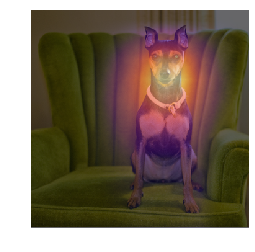
Looks similar to the previous non class-discriminative heatmap. Let’s run it for multiple inputs as before.
def plot_class_disc_multi(relu=True):
    random.seed(25)

    val_size = len(data.valid_ds)

    fig,ax = plt.subplots(2,4)
    fig.set_size_inches(12,6)

    for i in range(2):
        for j in range(0,4,2):
            idx=random.randint(0, val_size)
            x,y = data.valid_ds[idx]
            xb,_ = data.one_item(x)
            xb_im = Image(data.denorm(xb)[0])
            xb = xb.cuda()

            hook_a,hook_g = class_discriminative_activations(xb,y.data)
            acts = hook_a.stored[0].cpu()
            grad = hook_g.stored[0][0].cpu()

            grad_chan = grad.mean(1).mean(1)
            mult = (acts*grad_chan[...,None,None]).mean(0)

            if relu:
                mult = F.relu(mult)

            xb_im.show(ax[i,j])
            xb_im.show(ax[i,j+1])
            ax[i,j+1].imshow(mult, alpha=0.6, extent=(0,352,352,0),
                      interpolation='bilinear', cmap='magma');
    plt.show()
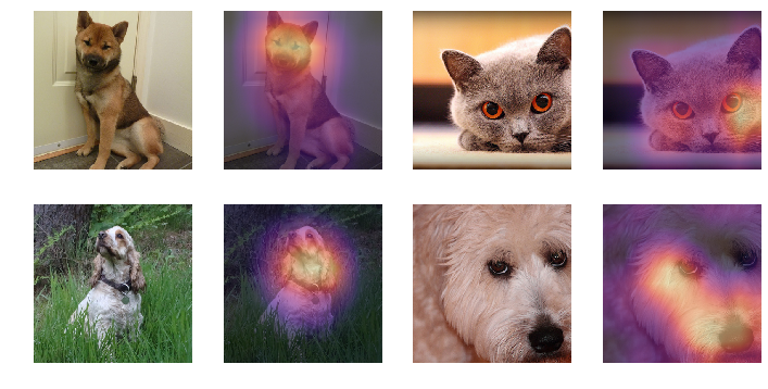
plot_class_disc_multi()
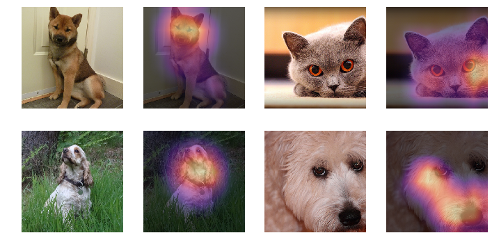
The heat-maps are more concentrated than before, and denote the specific features which led to an image being classified into a certain category.
Time to test it on the pug_maine.jpg image.
class_dict = {}
for i,el in enumerate(data.classes):
    class_dict[el.lower()] = i
show_class_discriminative_heatmap(x_test,class_dict['maine_coon'])
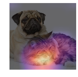
show_class_discriminative_heatmap(x_test,class_dict['pug'])
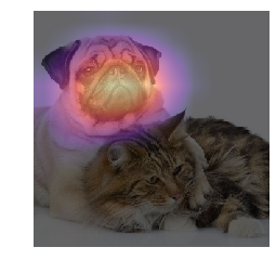
It works! The class-discriminative heat-map is only concentrated on the pixels specific to the class passed to the hook mechanism.
Let’s also check out the impact of performing a ReLU on the weighted combination of feature map activations and their importances. (ie, no ReLU on mult).
plot_class_disc_multi(relu=False)
As expected the heat-maps now highlight more than just the desired class. So ReLU only keeps the features that have a positive influence on the class of interest, and helps in achieving better localization.