This is the first post in this series on the basics of Machine Learning. My aim here is to create a comprehensive catalogue of ML concepts so that I can quickly refer to them in the future, as well as be of help to anybody in a position similar to mine.
This post complements the first segment in the zine: Linear Binary Classification. The idea is to have the content here supplement that in the zine.
The other posts in series can be found here.
Setup
!apt-get install imagemagick
!pip install -q celluloid
import matplotlib.pyplot as plt
import numpy as np
import pandas as pd
from celluloid import Camera
from IPython.display import HTML
wget -q https://gist.githubusercontent.com/dhth/38ab5621f61c1c2bf88320de9de32335/raw/fdeb5ebf14501f6235916321ba82cbae5bff12cf/linear-bin-classification.csv
def plot_points(X, y):
    dogs = X[np.argwhere(y==1)]
    cats = X[np.argwhere(y==0)]
    plt.scatter([s[0][0] for s in cats], [s[0][1] for s in cats], s = 25, color = 'red', edgecolor = 'k', label='cats')
    plt.scatter([s[0][0] for s in dogs], [s[0][1] for s in dogs], s = 25, color = 'blue', edgecolor = 'k', label='dogs')
    plt.xlabel('$x_1$')
    plt.ylabel('$x_2$')
    plt.legend()

def display(m, b, color='g--',label=None):
    plt.xlim(-0.05,1.05)
    plt.ylim(-0.05,1.05)
    x = np.arange(-10, 10, 0.1)
    plt.plot(x, m*x+b, color, label=label)
data = pd.read_csv('linear-bin-classification.csv', header=None)
fig = plt.figure()
X = np.array(data[[0,1]])
y = np.array(data[2])
plot_points(X,y)
plt.show()
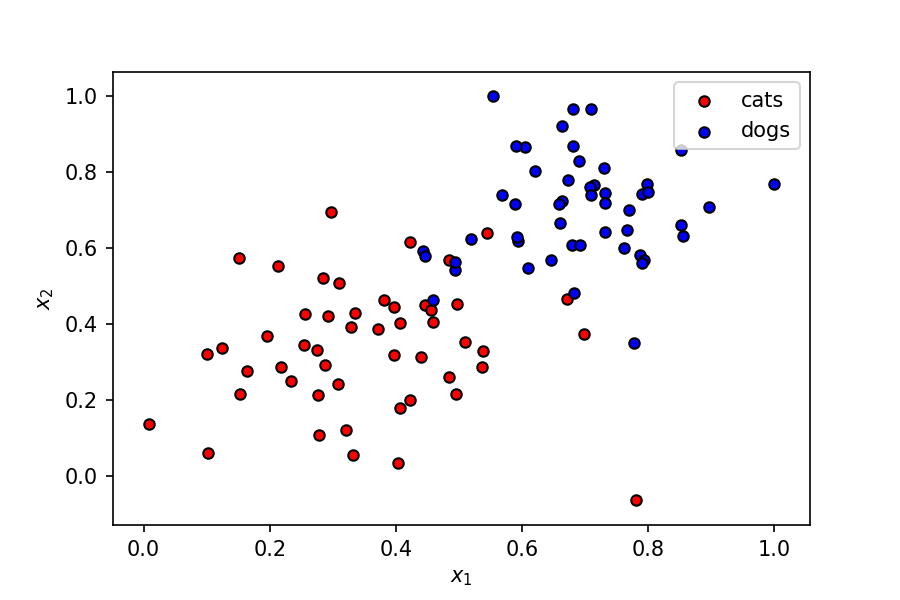
We’ve got a fairly simple dataset here, where two features (let’s call them $x_1$ and $x_2$) represent some characteristics of a pet, which can be a cat or a dog.
The dependent variable $y$ can have two values — $0$ or $1$ — corresponding to classes cat and dog respectively.
A linear boundary can easily separate the data points into two segments corresponding to the two classes. A perceptron is a good starting place to understand this problem.
Perceptron
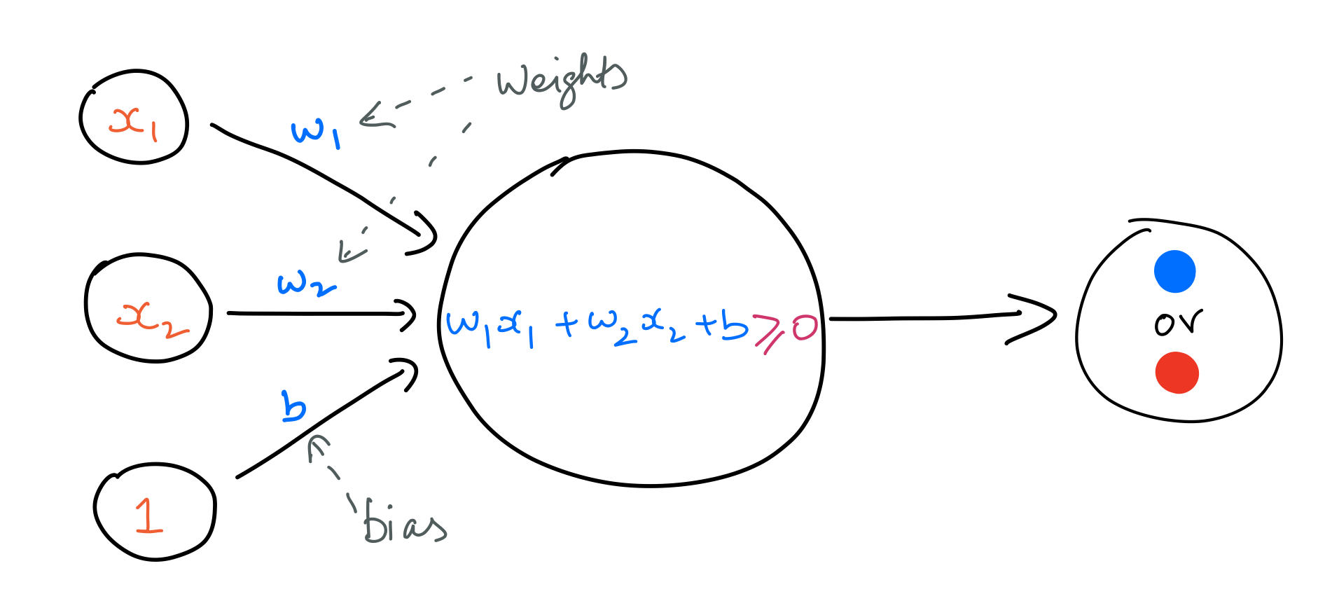
A perceptron is a particular kind of artificial neuron. It takes in an input vector and does a linear calculation as stated below. In this case, the input is a vector of length 2.
$$ \large lincalc = w_1x_1 + w_2x_2 + b $$
A perceptron uses the Heaviside step function to output binary values as outcomes. That is, if the value of lincalc is positive, the perceptron will output a $1$; and $0$ in the opposite case.
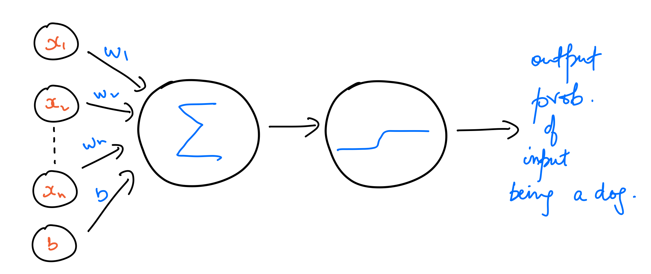
Neuron with sigmoid activation
A much better way of training models for binary classification is to work with output probabilities instead of binary values. To achieve that, we use a sigmoid function as the activation function instead of a step function. The output of this model is a probability of a data point belonging to the class dog, which corresponds to a $y$ value of $1$. Let’s call this output probability $\hat{y}$. That is,
$$ \large \hat{y} = sigmoid(w_1x_1 + w_2x_2 + b) $$
def sigmoid(x):
    return (1/(1+np.exp(-x)))

def output_formula(features, weights, bias):
    return sigmoid(np.matmul(features,weights) + bias)
Let’s see this in action. We’ll start with a random set of weights and bias set to zero.
np.random.seed(44)
weights = np.random.normal(scale=1 / 2**.5, size=2)
bias = 0
weights
array([-0.53076476, 0.93080519])
Next, we need to be able to visualize the linear boundary that this set of weights and bias corresponds to.
The equation of a line is:
$$ \large y = mx + c $$
where $m$ is the slope, and $c$ is the y intercept. The line corresponding to $ w_1x_1 + w_2x_2 + b = 0$ can be represented as:
$$ \large x_2 = -\frac{w_1}{w_2}x_1 - \frac{b}{w_2} $$
Let’s plot this line with the set of weights mentioned above.
fig=plt.figure()
plot_points(X,y)
display(-weights[0]/weights[1], -bias/weights[1], label=f'{"{0:.2f}".format(weights[0])}$x_1$ + {"{0:.2f}".format(weights[1])}$x_2$ + {bias} = 0')
plt.legend()
plt.show()
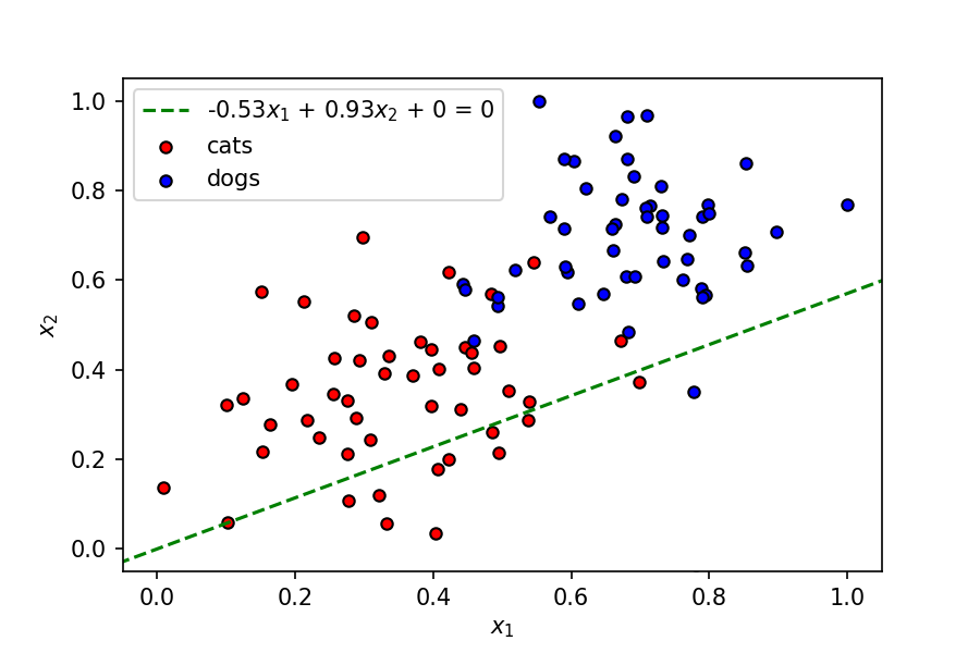
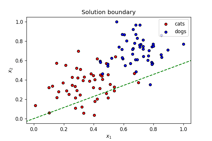
As seen above, this is not a great linear boundary for this dataset as it’s not doing a good job separating the data points into two clusters corresponding to the two classes. To improve this model, we need a metric to judge its accuracy; we do this using a loss function.
Loss Function
As stated before, the model will output the probability of an input feature vector belonging to the class dog. The loss function for this model should then return high values for bad predictions and low values for good predictions. In other words, if the model returns a value close to 1. for an input feature vector whose true class is dog, the loss for this prediction should be close to zero. In the opposite case, if the prediction for this vector is close to 0., the loss should be large.
The log function is a perfect candidate for this task. Let’s take a look at it’s graph.
x = np.linspace(1e-2,10,100)
fig, ax = plt.subplots()
ax.plot(x, np.log(x))
ax.grid(True, which='both')
ax.spines['left'].set_position('zero')
ax.spines['right'].set_color('none')
ax.yaxis.tick_left()
ax.spines['bottom'].set_position('zero')
ax.spines['top'].set_color('none')
ax.xaxis.tick_bottom()

fig.suptitle('y = log(x)', fontsize=20)
plt.show()
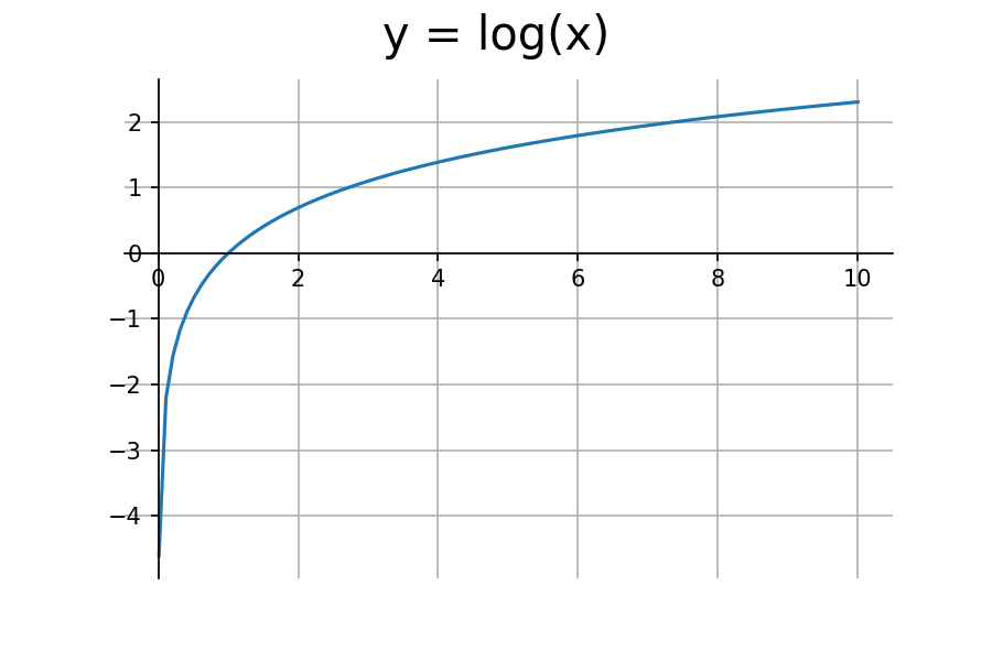
We’re only concerned with the input range of (0,1). The log function outputs negative values for this range. To get positive values, we need to multiply it by negative one.
x = np.linspace(1e-2,1.,100)
fig, ax = plt.subplots()
ax.plot(x, -np.log(x))
ax.grid(True, which='both')
ax.spines['left'].set_position('zero')
ax.spines['right'].set_color('none')
ax.yaxis.tick_left()
ax.spines['bottom'].set_position('zero')
ax.spines['top'].set_color('none')
ax.xaxis.tick_bottom()

fig.suptitle('y = -log(x)', fontsize=20)
plt.show()
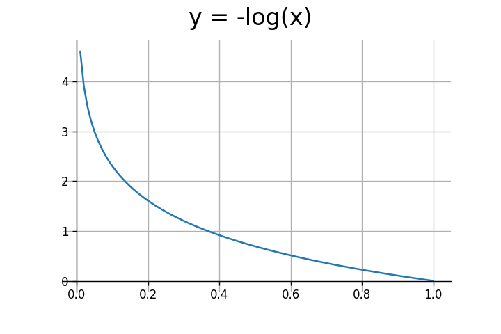
As seen above, the log function outputs large values for inputs closer to $0$, and small values for inputs closer to $1$. In the case of binary classification $y$ can either be $0$ or $1$. Let’s consider both scenarios.
In case of the true class being 0, we’d want the loss to be high if the output probability is close to $1$. $-\log(1-\hat{y})$ will result in high values if $\hat{y}$ is closer to $1$, and low values if if $\hat{y}$ is closer to $0$.
In case of the true class being 1, we’d want the loss to be high if the output probability is close to $0$. $-\log(\hat{y})$ will result in high values if $\hat{y}$ is closer to $0$, and low values if if $\hat{y}$ is closer to $1$.
The two cases are encapsulated into a single equation by the binary cross entropy loss function, which is defined for a single data point as:
$$ \large E = -y\log(\hat{y}) - (1-y)\log(1-\hat{y}) $$
- In case of the true class being 0, the first term will amount to
zero. - In case of the true class being 1, the second term will amount to
zero.
Loss (or Error) for all data points is simply the mean of individual losses:
$$ \large E = - \frac{1}{m}\sum_{i=1}^{m}[y_i\log(\hat{y_i}) + (1-y_i)\log(1-\hat{y_i})] $$
A more comprehensive analysis of the binary cross entropy function can be found here. Let’s check out the loss for the set of weights used above.
def error_formula(y, output):
    return -1*y*np.log(output) - (1-y)*np.log(1-output)
out = output_formula(X, weights, bias)
loss = np.mean(error_formula(y, out))
out.shape, loss
((100,), 0.6625515973520308)
Next, we need to optimise the parameters of the model — the weights and the bias — to minimise this loss. We’ll do that using gradient descent.
Gradient Descent
Since the error is a function of $w_1$, $w_2$, and $b$, it can be minimised by following the gradient descent rule as follows:
$$ \large w_1 \leftarrow w_1 - \alpha\frac{\partial E}{\partial w_1} $$
$$ \large w_2 \leftarrow w_2 - \alpha\frac{\partial E}{\partial w_2} $$
$$ \large b \leftarrow b - \alpha\frac{\partial E}{\partial b} $$
where $\alpha$ is the learning rate.
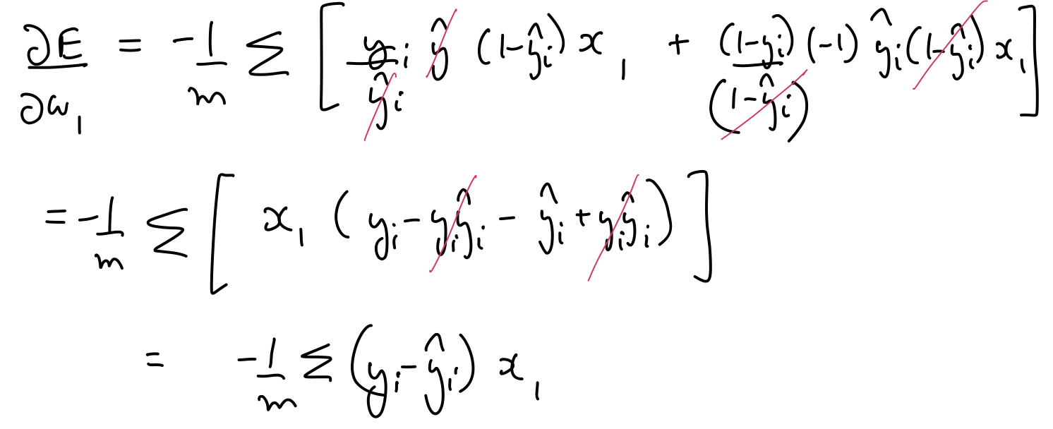
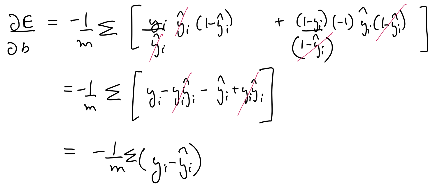
$\frac{\partial E}{\partial w_1}$, $\frac{\partial E}{\partial w_2}$, $\frac{\partial E}{\partial b}$ can be calculated as follows:
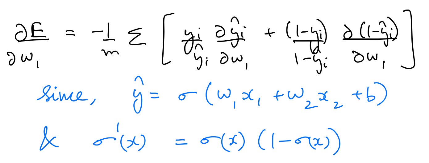
Thus, the parameters need to be updated as follows:
$$ \large w_j \leftarrow w_j + \frac{\alpha}{m}\sum_{i=1}^{m}(y_i - \hat{y_i})x_j $$
$$ \large b \leftarrow b + \frac{\alpha}{m}\sum_{i=1}^{m}(y_i - \hat{y_i}) $$
def update_weights(x, y, weights, bias, learnrate):
    out = output_formula(x,weights,bias)
    weights += learnrate*(y-out)*x
    bias += learnrate*(y-out)
    return weights,bias
Training
Putting all of this together in a single function:
np.random.seed(44)

epochs = 100
learnrate = 0.01

def train(features, targets, epochs, learnrate, graph_lines=False, print_stats=False):

    fig = plt.figure(dpi=120)
    camera = Camera(fig)
    errors = []
    n_records, n_features = features.shape
    last_loss = None
    weights = np.random.normal(scale=1 / n_features**.5, size=n_features)
    bias = 0
    display(-weights[0]/weights[1], -bias/weights[1])
    camera.snap()
    for e in range(epochs):
        del_w = np.zeros(weights.shape)
        for x, y in zip(features, targets):
            output = output_formula(x, weights, bias)
            error = error_formula(y, output)
            weights, bias = update_weights(x, y, weights, bias, learnrate)

        out = output_formula(features, weights, bias)
        loss = np.mean(error_formula(targets, out))
        errors.append(loss)
        if print_stats:
            if e % (epochs / 10) == 0:
                print("\n========== Epoch", e,"==========")
                if last_loss and last_loss < loss:
                    print("Train loss: ", loss, "  WARNING - Loss Increasing")
                else:
                    print("Train loss: ", loss)
                last_loss = loss
                predictions = out > 0.5
                accuracy = np.mean(predictions == targets)
                print("Accuracy: ", accuracy)
        if graph_lines and e % (epochs / 100) == 0:
            display(-weights[0]/weights[1], -bias/weights[1])
            plt.text(.1, 0.95 ,f'Loss: {"{0:.2f}".format(loss)}',
             horizontalalignment='center',
             verticalalignment='center')
            camera.snap()

    plt.title("Solution boundary")
    plot_points(features, targets)
    plt.show()
    animation = camera.animate()
    animation.save('5.gif', writer = 'imagemagick')

    return animation
anim = train(X, y, epochs, learnrate, True, False)
HTML(anim.to_html5_video())