This is the third post in this series on the basics of Machine Learning. In the last one, we learnt how a Multilayer Perceptron can be trained to non-linearly segment a dataset. We also saw how a simple artificial neuron forms the building block of a Multilayer Perceptron — or a neural network in general — which can learn much more complicated decision boundaries.
Let’s move on to datasets that are harder to segment. One way to improve the learning capability of a MLP is to add more neurons in the form of hidden layers. In this post we’ll explore MLPs with 2 hidden layers.
Setup
!apt-get -q install imagemagick
!pip install -q celluloid
from sklearn.datasets import make_classification, make_circles, make_moons, make_blobs,make_checkerboard
import matplotlib.pyplot as plt
import numpy as np
import pandas as pd
from IPython.display import HTML
import pickle
from math import ceil
from matplotlib.offsetbox import AnchoredText
from celluloid import Camera
def plot_points(X, y, alpha=None):
    dogs = X[np.argwhere(y==1)]
    cats = X[np.argwhere(y==0)]
    plt.scatter([s[0][0] for s in cats], [s[0][1] for s in cats], s = 25, \
                color = 'red', edgecolor = 'k', label='cat', alpha=alpha)
    plt.scatter([s[0][0] for s in dogs], [s[0][1] for s in dogs], s = 25, \
                color = 'blue', edgecolor = 'k', label='dog', alpha=alpha)
    plt.xlabel('$x_1$')
    plt.ylabel('$x_2$')
    plt.legend()
Let’s use a new dataset for this exercise.
wget -q https://gist.githubusercontent.com/dhth/fcd27938c26dbc6124c1c70646a52cfc/raw/2fabb32c1008afefeaf006fcf7602638de0c8699/exor_dataset.csv
data = pd.read_csv('exor_dataset.csv', header=None)
fig = plt.figure(dpi=120)
X = np.array(data[[0,1]])
y = np.array(data[2]).astype(int)
plot_points(X,y)
plt.xlim(X[:,0].min()-0.5,X[:,0].max()+0.5)
plt.ylim(X[:,1].min()-0.5,X[:,1].max()+0.5)
plt.savefig('1.png')
plt.show()
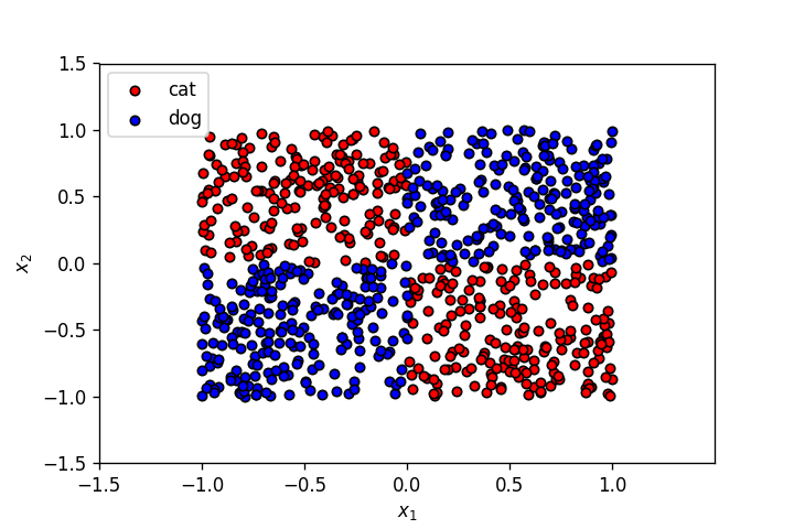
The labels of the points above have an EX-OR relationship with the input features.
Let’s start by training the MLP from the last post on this dataset. Copying the same functions from last time:
def sigmoid(x):
    return 1/(1+np.exp(-x))
class MLPNeuralNet(object):
    def __init__(self,N_input, N_hidden,N_output):
        self.weights_input_to_hidden = np.random.normal(0, scale=0.1, size=(N_input, N_hidden))
        self.weights_hidden_to_output = np.random.normal(0, scale=0.1, size=(N_hidden, N_output))

        self.bias_input_to_hidden = np.zeros(N_hidden)
        self.bias_hidden_to_output = np.zeros(N_output)

    def feed_forward(self,input_x):
        self.hidden_layer_in = np.dot(input_x,self.weights_input_to_hidden) + self.bias_input_to_hidden
        self.hidden_layer_out = sigmoid(self.hidden_layer_in)
        self.output_layer_in = np.dot(self.hidden_layer_out,self.weights_hidden_to_output) + self.bias_hidden_to_output
        self.output_layer_out = sigmoid(self.output_layer_in)
        return self.output_layer_out

    def get_hidden_layer_in(self,input_x):
        return np.dot(input_x,self.weights_input_to_hidden) + self.bias_input_to_hidden

    def get_output_layer_in(self,input_x):
        self.hidden_layer_in = np.dot(input_x,self.weights_input_to_hidden) + self.bias_input_to_hidden
        self.hidden_layer_out = sigmoid(self.hidden_layer_in)
        return np.dot(self.hidden_layer_out,self.weights_hidden_to_output) + self.bias_hidden_to_output

    def back_propagate(self,input_x,output_y, learn_rate):
        error = (-1)*(output_y*np.log(self.output_layer_out) + (1-output_y)*np.log(1-self.output_layer_out))
        del_y_out = (-1)*output_y/self.output_layer_out + (1-output_y)/(1-self.output_layer_out)
        del_h = del_y_out*self.output_layer_out*(1-self.output_layer_out)*self.weights_hidden_to_output.T
        del_w_h_o = del_y_out*self.output_layer_out*(1-self.output_layer_out)*self.hidden_layer_out.T
        del_b_o = del_y_out*self.output_layer_out*(1-self.output_layer_out)
        del_w_i_h = del_h*self.hidden_layer_out*(1-self.hidden_layer_out)*input_x.T
        del_b_h = del_h*self.hidden_layer_out*(1-self.hidden_layer_out)

        self.weights_hidden_to_output -= learn_rate*del_w_h_o
        self.bias_hidden_to_output -= learn_rate*del_b_o[0,:]

        self.weights_input_to_hidden -= learn_rate*del_w_i_h
        self.bias_input_to_hidden -= learn_rate*del_b_h[0,:]
        return error
def train(nn, features, outputs, num_epochs, learn_rate, print_error=False):

    for e in range(num_epochs):
        for input_x, output_y in zip(features, outputs):
            input_x = input_x.reshape(1,-1)
            output_y = output_y.reshape(1,-1)

            output_layer_out = nn.feed_forward(input_x)

            error = nn.back_propagate(input_x,output_y,learn_rate=learn_rate)

        if print_error:
            if e%200==0:
                print(error[0][0])
def display_linear_boundary(ax, m, b, x_1_lims,x_2_lims,color='g--',label=None,linewidth=3.):
    ax.set_xlim(x_1_lims)
    ax.set_ylim(x_2_lims)
    x = np.arange(-10, 10, 0.1)
    ax.plot(x, m*x+b, color, label=label,linewidth=linewidth)
    ax.set_yticklabels([])
    ax.set_xticklabels([])
    return ax
def plot_points_on_ax(ax,X, y,alpha):
    dogs = X[np.argwhere(y==1)]
    cats = X[np.argwhere(y==0)]
    ax.scatter([s[0][0] for s in cats], [s[0][1] for s in cats], s = 25, \
               color = 'red', edgecolor = 'k', label='cats',alpha=alpha)
    ax.scatter([s[0][0] for s in dogs], [s[0][1] for s in dogs], s = 25, \
               color = 'blue', edgecolor = 'k', label='dogs',alpha=alpha)
    return ax
def create_decision_boundary_anim(nn,X,y,epochs=300,learn_rate=1e-3,snap_every=100,dpi=100,print_error=False, num_cols=2):

    hidden_units = nn.weights_hidden_to_output.shape[0]

    num_subplots = 1 + hidden_units

    num_rows = ceil(num_subplots/num_cols)

    fig,axes = plt.subplots(num_rows, num_cols, figsize=(num_cols*3,num_rows*3),dpi=dpi)

    axes_list = list(axes.flat)

    for ax in axes.flat:
        ax.set_yticklabels([])
        ax.set_xticklabels([])
        ax.get_xaxis().set_visible(False)
        ax.get_yaxis().set_visible(False)

    final_dec_boundary_ax = axes_list[0]

    hidden_layer_ax = axes_list[1:hidden_units+1]

    camera = Camera(fig)

    h = .02

    x_min, x_max = X[:, 0].min() - 0.5, X[:, 0].max() + 0.5
    y_min, y_max = X[:, 1].min() - 0.5, X[:, 1].max() + 0.5
    xx, yy = np.meshgrid(np.arange(x_min, x_max, h),
                     np.arange(y_min, y_max, h))

    for e in range(ceil(epochs/snap_every)):
        train(nn,X,y,snap_every,learn_rate,print_error=print_error)
        Z = (nn.feed_forward(np.c_[xx.ravel(), yy.ravel()]) >0.5).astype(int)
        Z = Z.reshape(xx.shape)
        final_dec_boundary_ax.contourf(xx, yy, Z, cmap=plt.cm.RdBu)

        text_box = AnchoredText(f'Epoch: {snap_every*(e+1)}', frameon=True, loc=4, pad=0.5)
        plt.setp(text_box.patch, facecolor='white', alpha=0.5)
        final_dec_boundary_ax.add_artist(text_box)

        Z_hidden = (nn.get_hidden_layer_in(np.c_[xx.ravel(), yy.ravel()]) >=0.).astype(int)

        for i,ax in enumerate(hidden_layer_ax):
            Z_ = Z_hidden[:,i].reshape(-1,1)
            Z_ = Z_.reshape(xx.shape)
            ax.contourf(xx, yy, Z_, cmap=plt.cm.RdBu)

        camera.snap()

    final_dec_boundary_ax = plot_points_on_ax(final_dec_boundary_ax,X, y,alpha=.6)
    final_dec_boundary_ax.set_title(f'Decision boundary of MLP')

    for i,ax in enumerate(hidden_layer_ax):
        ax = plot_points_on_ax(ax,X, y,alpha=.6)
        ax.set_title(f'Hidden neuron {i+1}')

    plt.annotate('https://dhruvs.space', xy=(1, 0), xycoords='axes fraction', fontsize=9,
                xytext=(0, -15), textcoords='offset points',
                ha='right', va='top')
    plt.tight_layout()
    animation = camera.animate()

    return animation
np.random.seed(10)
nn = MLPNeuralNet(2, 3, 1)

anim = create_decision_boundary_anim(nn,X,y,\
                                     epochs=300,dpi=40,\
                                     learn_rate=5e-2,snap_every=50,\
                                     print_error=True)
plt.close()
HTML(anim.to_html5_video())

The gif above shows the decision boundaries of the MLP as a whole, as well as those of the hidden neurons. As evident from it, this MLP with a single hidden layer is having a hard time segmenting this dataset. It can be achieved — with proper weight initialisation, adding custom input features ($x_1\times x_2$), and by making use of other activation functions — but that’s not the point here. An MLP with a single hidden layer will eventually prove to be insufficient as the complexity of the dataset increases. Let’s add another layer of hidden neurons to this MLP, and see if that helps.
Multilayer Perceptron with 3 layers
The following is a MLP with 2 hidden layers.
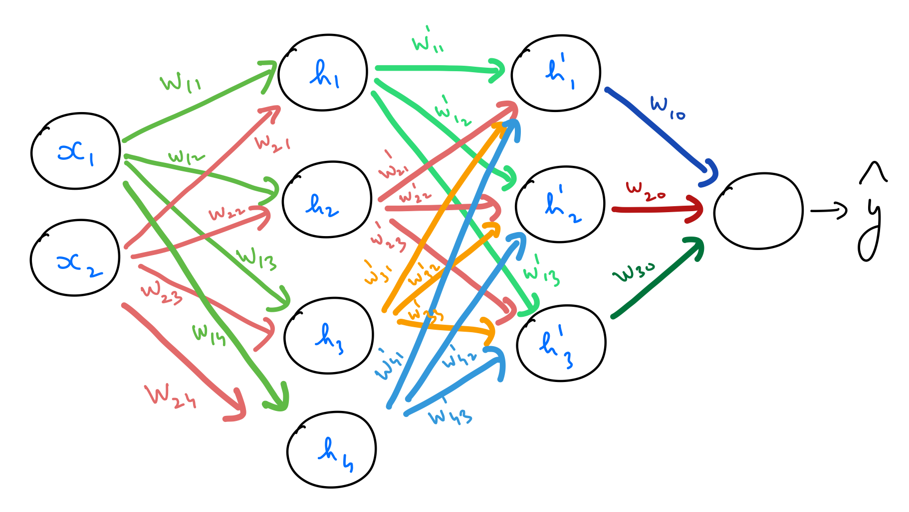
Feedforward
Let’s go through the process step by step, as before.
input_x = X[0,:].reshape(1,-1)
output_y = y[0].reshape(1,-1)
input_x.shape, output_y.shape
((1, 2), (1, 1))
N_input = 2
N_hidden_1 = 4
N_hidden_2 = 3
N_output = 1
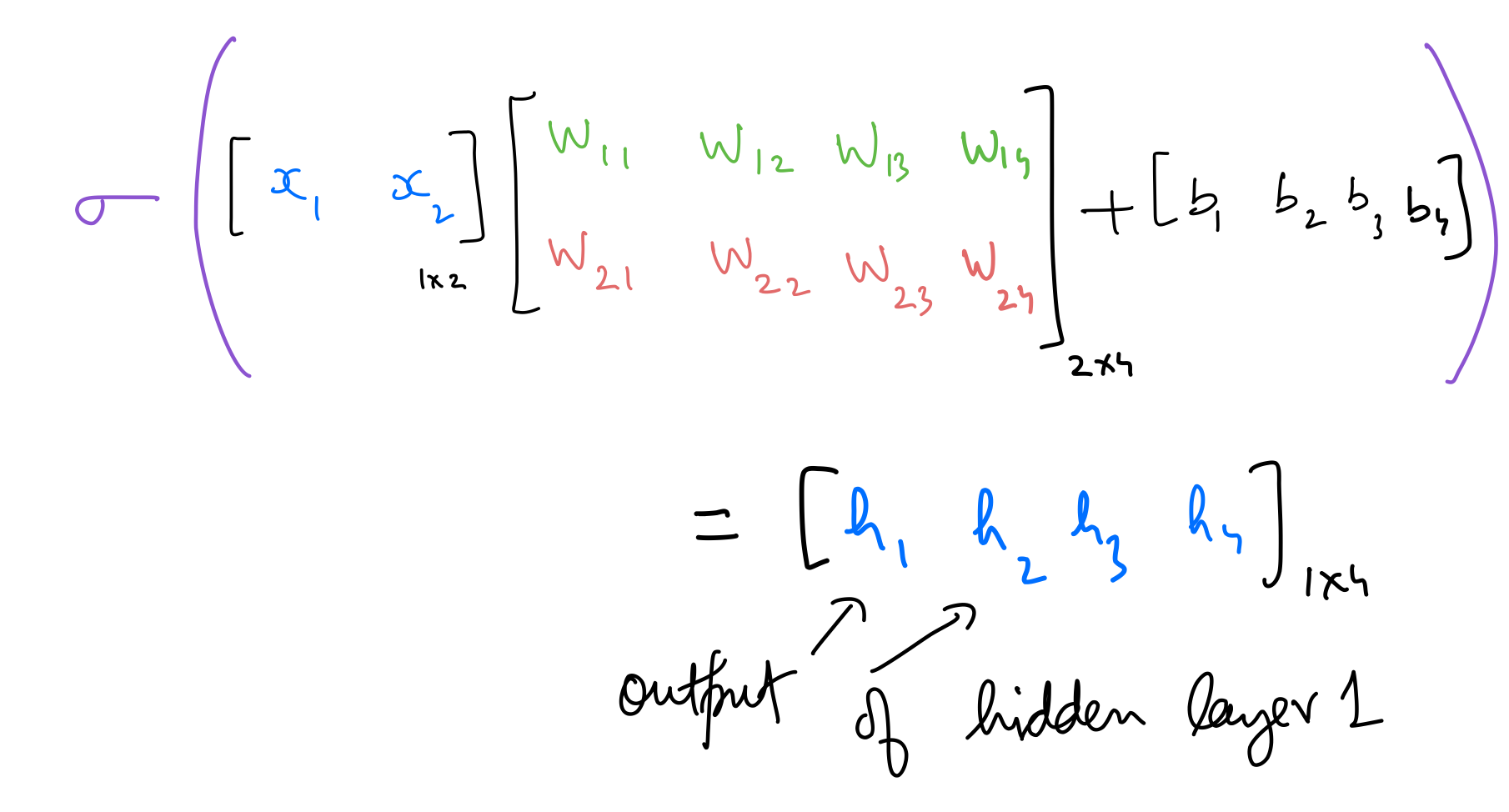
This time we’ll initialize the weights in a different way. We’ll randomly select values from a normal distribution and then multipy them by the factor: $$ \large \sqrt{\frac{2}{\text{outputTensor.shape[1]}}} $$
I’ll get into the reasoning behind this kind of initialization in an upcoming post. This approach is called Xavier initialisation. More details about this approach can be found here and here.
We’ll be needing 3 sets of weights this time.
$$ \large \text{weightsInputToHidden} = \begin{bmatrix} w_{11} & w_{12} & w_{13} & w_{14}\ w_{21} & w_{22} & w_{23} & w_{24} \end{bmatrix} $$
weights_input_to_hidden_1 = np.random.randn(N_input, N_hidden_1)*np.sqrt(1/N_hidden_1)
weights_input_to_hidden_1
array([[-0.87295171, -0.39113499,  0.21779305, -0.18998006],
       [ 0.34119755,  0.36595149,  0.15416373,  0.4653826 ]])
weights_hidden_1_to_hidden_2 = np.random.randn(N_hidden_1, N_hidden_2)*np.sqrt(1/N_hidden_2)
weights_hidden_1_to_hidden_2
array([[ 0.17291965, -0.17246838,  0.19489309],
       [ 0.4630033 ,  0.02347373, -0.17954312],
       [ 0.12243623,  0.26875939, -1.28381417],
       [ 0.63412901, -0.52092003,  0.93676923]])
weights_hidden_2_to_output = np.random.randn(N_hidden_2, N_output)*np.sqrt(1/N_output)
weights_hidden_2_to_output
array([[ 1.19416008],
       [ 1.34523525],
       [-0.42948187]])
We need 3 sets of biases as well. $$ \large \text{biasHidden1} =\begin{bmatrix} b_{1}&b_{2}&b_{3}&b_{4} \end{bmatrix} $$
bias_input_to_hidden_1 = np.zeros(N_hidden_1)
bias_input_to_hidden_1
array([0., 0., 0., 0.])
$$ \large \text{biasHidden2} =\begin{bmatrix} b^{’}{1}&b^{’}{2}&b^{’}_{3} \end{bmatrix} $$
bias_hidden_1_to_hidden_2 = np.zeros(N_hidden_2)
bias_hidden_1_to_hidden_2
array([0., 0., 0.])
$$ \large \text{biasOut} =\begin{bmatrix} b_{0} \end{bmatrix} $$
bias_hidden_2_to_output = np.zeros(N_output)
bias_hidden_2_to_output
array([0.])
The difference this time is that we need to perform one more set of calculations — for both feedforward, and backpropagation stages — corresponding to the added hidden layer.
Hidden 1 out
hidden_layer_1_in = np.dot(input_x,weights_input_to_hidden_1) + bias_input_to_hidden_1
hidden_layer_1_in.shape
(1, 4)
hidden_layer_1_out = sigmoid(hidden_layer_1_in)
hidden_layer_1_out.shape
(1, 4)
Hidden 2 out
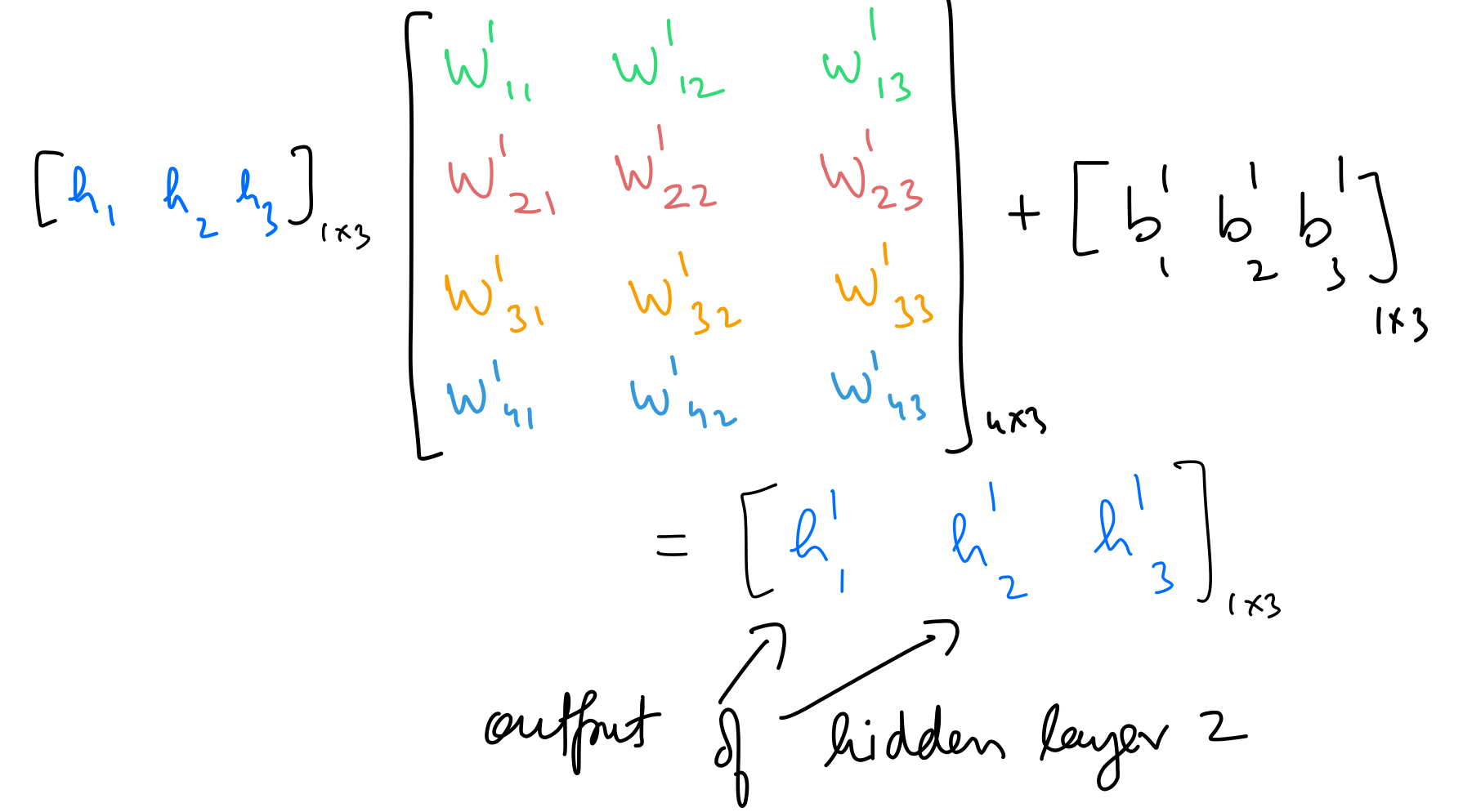
hidden_layer_2_in = np.dot(hidden_layer_1_out,weights_hidden_1_to_hidden_2) + bias_hidden_1_to_hidden_2
hidden_layer_2_in.shape
(1, 3)
hidden_layer_2_out = sigmoid(hidden_layer_2_in)
hidden_layer_2_out.shape
(1, 3)
Output
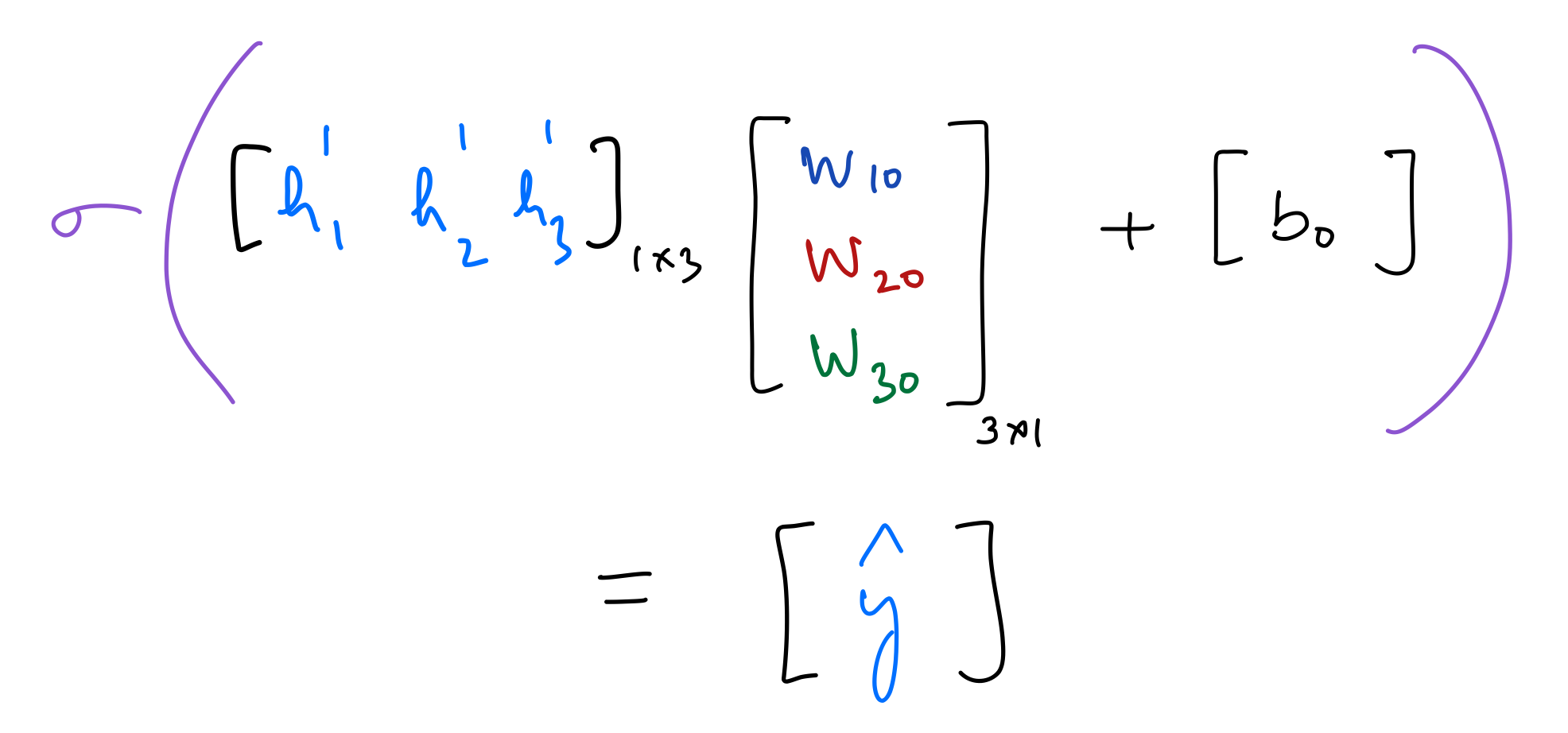
output_layer_in = np.dot(hidden_layer_2_out,weights_hidden_2_to_output) + bias_hidden_2_to_output
output_layer_in.shape
(1, 1)
output_layer_out = sigmoid(output_layer_in)
output_layer_out.shape
(1, 1)
Error
error = (-1)*(output_y*np.log(output_layer_out) + (1-output_y)*np.log(1-output_layer_out))
error
array([[1.30734966]])
Backpropagation
Calculating the partial derivatives wrt. the error.
Partial derivative wrt prediction
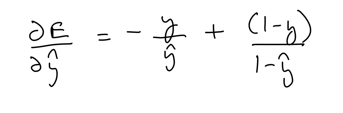
del_y_out = (-1)*output_y/output_layer_out + (1-output_y)/(1-output_layer_out)
assert del_y_out.shape == output_layer_out.shape
del_y_out
array([[3.69636411]])
Partial derivative wrt hidden layer 2 out
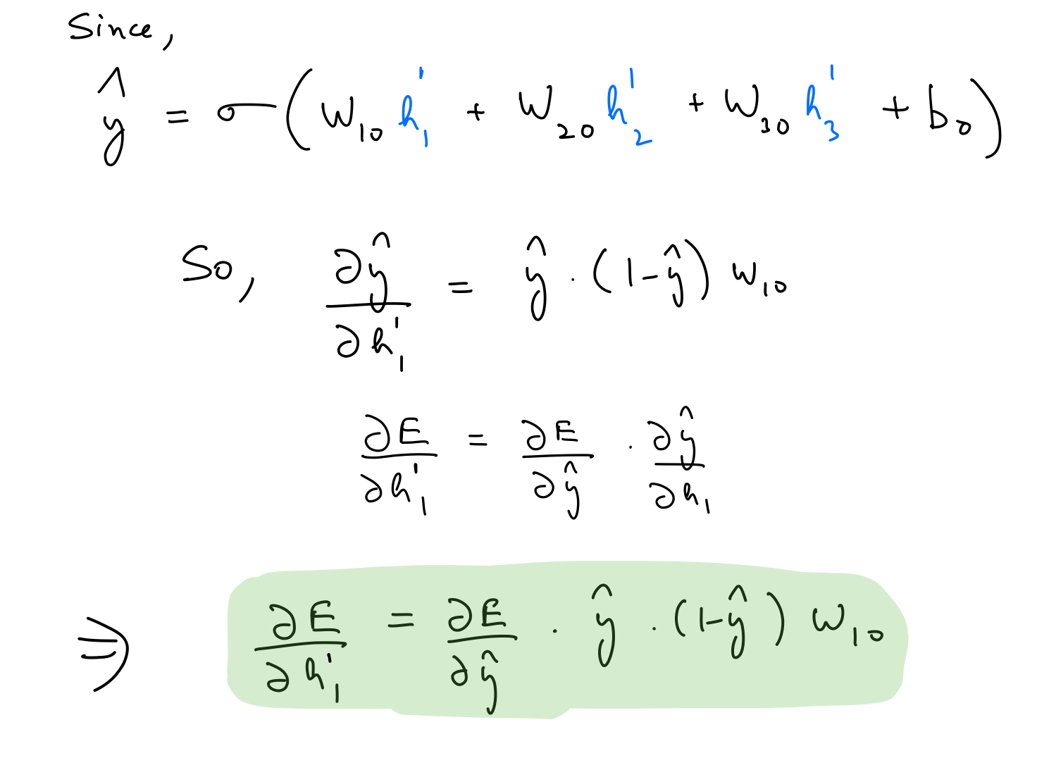
del_h_2 = del_y_out*output_layer_out*(1-output_layer_out)*weights_hidden_2_to_output.T
assert del_h_2.shape == hidden_layer_2_out.shape
del_h_2
array([[ 0.98222332, 0.69578643, -0.18424711]])
Partial derivative wrt output layer weights
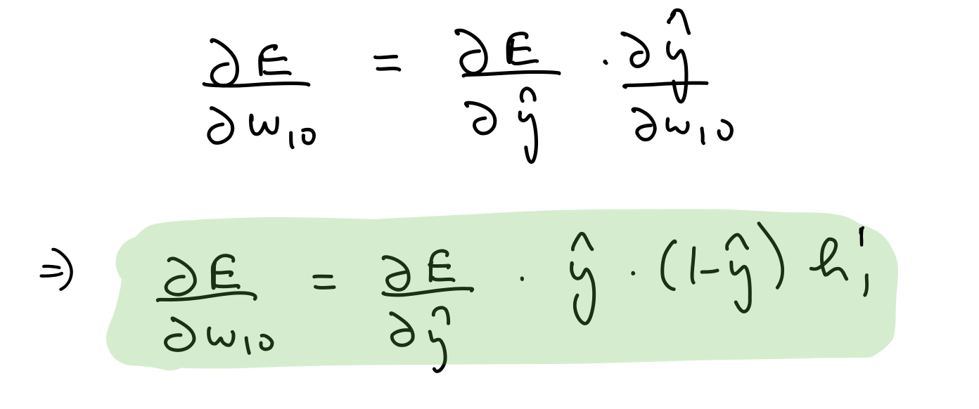
del_w_h_2_o = del_y_out*output_layer_out*(1-output_layer_out)*hidden_layer_2_out.T
assert del_w_h_2_o.shape == weights_hidden_2_to_output.shape
del_w_h_2_o
array([[0.38490508],
       [0.33039262],
       [0.43493646]])
Partial derivative wrt output layer biases
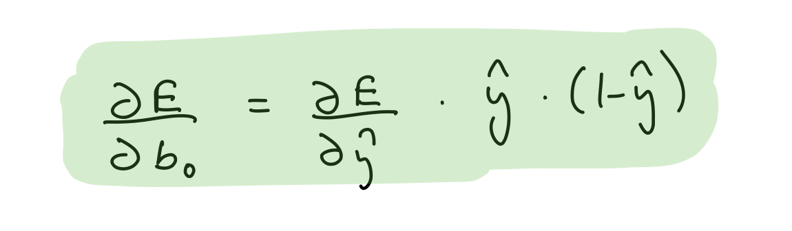
del_b_2_o = (del_y_out*output_layer_out*(1-output_layer_out))[0]
assert del_b_2_o.shape == bias_hidden_2_to_output.shape
del_b_2_o
Partial derivative wrt hidden layer 1 out
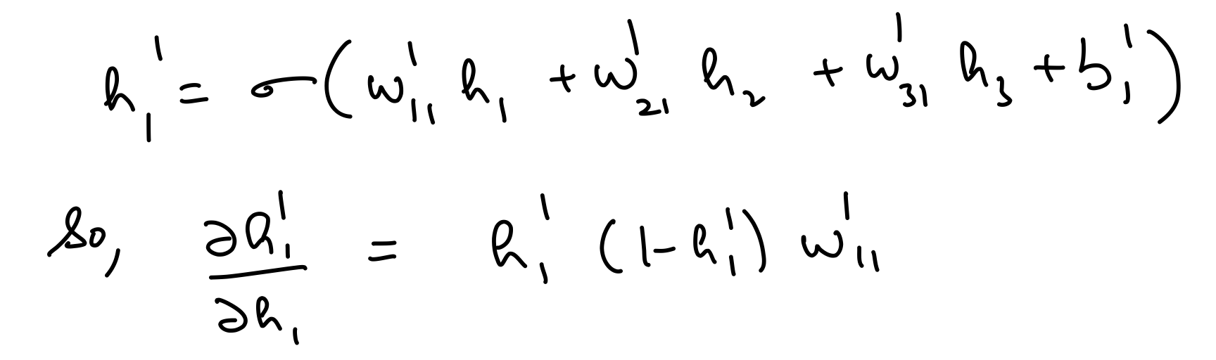
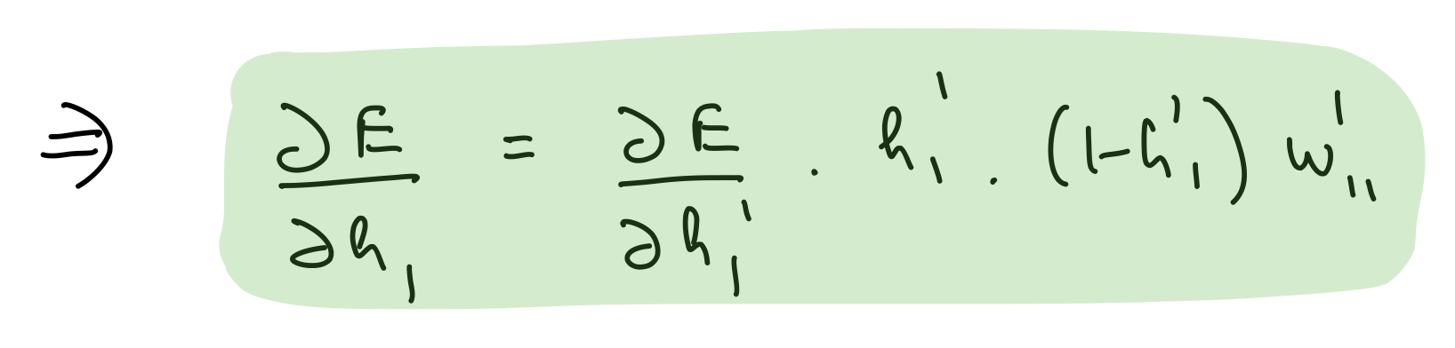
del_h_1 = np.dot(del_h_2*hidden_layer_2_out*(1-hidden_layer_2_out),weights_hidden_1_to_hidden_2.T)
assert del_h_1.shape == hidden_layer_1_out.shape
del_h_1
array([[-0.0099859 , 0.21296845, -0.25630071, 0.02174339]])
Partial derivative wrt hidden layer 2 weights

del_w_h_1_h_2 = del_h_2*hidden_layer_2_out*(1-hidden_layer_2_out)*hidden_layer_1_out.T
assert del_w_h_1_h_2.shape == weights_hidden_1_to_hidden_2.shape
del_w_h_1_h_2
array([[ 0.13521625,  0.09522663, -0.02449931],
       [ 0.10612383,  0.07473816, -0.01922817],
       [ 0.11346658,  0.07990933, -0.02055857],
       [ 0.10408398,  0.07330159, -0.01885857]])
Partial derivative wrt hidden layer 2 biases

del_b_h_1_h_2 = (del_h_2*hidden_layer_2_out*(1-hidden_layer_2_out))[0]
assert del_b_h_1_h_2.shape == bias_hidden_1_to_hidden_2.shape
del_b_h_1_h_2
array([ 0.24480464, 0.17240472, -0.04435521])
Partial derivative wrt hidden layer 1 weights
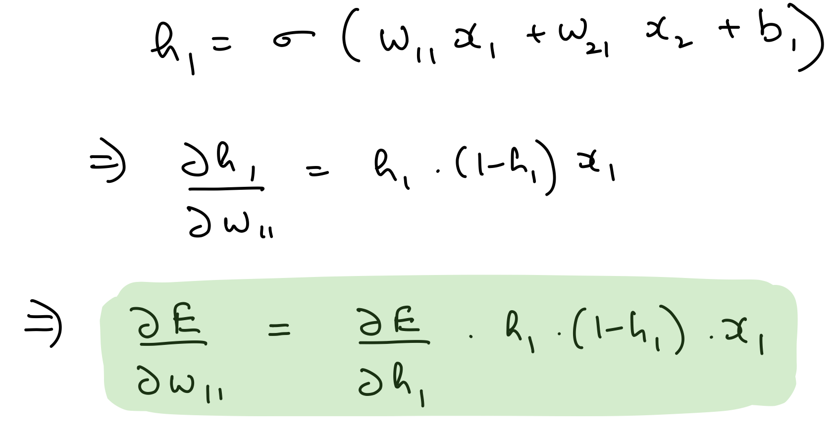
del_w_i_h_1 = del_h_1*hidden_layer_1_out*(1-hidden_layer_1_out)*input_x.T
assert del_w_i_h_1.shape == weights_input_to_hidden_1.shape
del_w_i_h_1
array([[-0.0013237 ,  0.02803837, -0.03416776,  0.0028489 ],
       [ 0.00153643, -0.03254447,  0.03965893, -0.00330675]])
Partial derivative wrt hidden layer 1 biases

del_b_i_h_1 = (del_h_1*hidden_layer_1_out*(1-hidden_layer_1_out))[0]
assert del_b_i_h_1.shape == bias_input_to_hidden_1.shape
del_b_i_h_1
array([-0.00246912, 0.05230043, -0.06373369, 0.0053141 ])
learn_rate = 1e-3
weights_hidden_2_to_output -= learn_rate*del_w_h_2_o
bias_hidden_2_to_output -= learn_rate*del_b_2_o

weights_hidden_1_to_hidden_2 -= learn_rate*del_w_h_1_h_2
bias_hidden_1_to_hidden_2 -= learn_rate*del_b_h_1_h_2

weights_input_to_hidden_1 -= learn_rate*del_w_i_h_1
bias_input_to_hidden_1 -= learn_rate*del_b_i_h_1
Putting all of this in a single class. I’ve also added the function get_hidden_layer_outputs to get intermediate activations from the MLP.
class MLPNeuralNet3Layers(object):
    def __init__(self,N_input, N_hidden_1, N_hidden_2, N_output):

        self.weights_input_to_hidden_1 = np.random.randn(N_input, N_hidden_1)*np.sqrt(1/N_hidden_1)
        self.weights_hidden_1_to_hidden_2 = np.random.randn(N_hidden_1, N_hidden_2)*np.sqrt(1/N_hidden_2)
        self.weights_hidden_2_to_output = np.random.randn(N_hidden_2, N_output)*np.sqrt(1/N_output)

        self.bias_input_to_hidden_1 = np.zeros(N_hidden_1)
        self.bias_hidden_1_to_hidden_2 = np.zeros(N_hidden_2)
        self.bias_hidden_2_to_output = np.zeros(N_output)

    def feed_forward(self,input_x):
        self.hidden_layer_1_in = np.dot(input_x,self.weights_input_to_hidden_1) + self.bias_input_to_hidden_1
        self.hidden_layer_1_out = sigmoid(self.hidden_layer_1_in)
        self.hidden_layer_2_in = np.dot(self.hidden_layer_1_out,self.weights_hidden_1_to_hidden_2) + self.bias_hidden_1_to_hidden_2
        self.hidden_layer_2_out = sigmoid(self.hidden_layer_2_in)
        self.output_layer_in = np.dot(self.hidden_layer_2_out,self.weights_hidden_2_to_output) + self.bias_hidden_2_to_output
        self.output_layer_out = sigmoid(self.output_layer_in)

        return self.output_layer_out

    def get_hidden_layer_outputs(self,input_x):
        self.hidden_layer_1_in = np.dot(input_x,self.weights_input_to_hidden_1) + self.bias_input_to_hidden_1
        self.hidden_layer_1_out = sigmoid(self.hidden_layer_1_in)
        self.hidden_layer_2_in = np.dot(self.hidden_layer_1_out,self.weights_hidden_1_to_hidden_2) + self.bias_hidden_1_to_hidden_2

        return (self.hidden_layer_1_in,self.hidden_layer_2_in)

    def back_propagate(self,input_x,output_y, learn_rate):
        error = (-1)*(output_y*np.log(self.output_layer_out) + (1-output_y)*np.log(1-self.output_layer_out))
        del_y_out = (-1)*output_y/self.output_layer_out + (1-output_y)/(1-self.output_layer_out)

        del_h_2 = del_y_out*self.output_layer_out*(1-self.output_layer_out)*self.weights_hidden_2_to_output.T
        del_w_h_2_o = del_y_out*self.output_layer_out*(1-self.output_layer_out)*self.hidden_layer_2_out.T
        del_b_2_o = (del_y_out*self.output_layer_out*(1-self.output_layer_out))[0]

        del_h_1 = np.dot(del_h_2*self.hidden_layer_2_out*(1-self.hidden_layer_2_out),self.weights_hidden_1_to_hidden_2.T)
        del_w_h_1_h_2 = del_h_2*self.hidden_layer_2_out*(1-self.hidden_layer_2_out)*self.hidden_layer_1_out.T
        del_b_h_1_h_2 = (del_h_2*self.hidden_layer_2_out*(1-self.hidden_layer_2_out))[0]

        del_w_i_h_1 = del_h_1*self.hidden_layer_1_out*(1-self.hidden_layer_1_out)*input_x.T
        del_b_i_h_1 = (del_h_1*self.hidden_layer_1_out*(1-self.hidden_layer_1_out))[0]

        self.weights_hidden_2_to_output -= learn_rate*del_w_h_2_o
        self.bias_hidden_2_to_output -= learn_rate*del_b_2_o

        self.weights_hidden_1_to_hidden_2 -= learn_rate*del_w_h_1_h_2
        self.bias_hidden_1_to_hidden_2 -= learn_rate*del_b_h_1_h_2

        self.weights_input_to_hidden_1 -= learn_rate*del_w_i_h_1
        self.bias_input_to_hidden_1 -= learn_rate*del_b_i_h_1

        return error
Decision Boundaries
Let’s train this MLP and see the evolution of decision boundaries of the MLP itself, as well as the constituent neurons. We can use the same train function from before.
def create_decision_boundary_anim(nn,X,y,epochs=300,learn_rate=1e-3,snap_every=100,dpi=100,print_error=False, num_cols=2):

    hidden_layer_1_units = nn.weights_hidden_1_to_hidden_2.shape[0]
    hidden_layer_2_units = nn.weights_hidden_2_to_output.shape[0]

    num_subplots = 1 + hidden_layer_1_units + hidden_layer_2_units

    num_rows = ceil(num_subplots/num_cols)

    fig,axes = plt.subplots(num_rows, num_cols, figsize=(num_cols*3,num_rows*3),dpi=dpi)

    axes_list = list(axes.flat)

    for ax in axes.flat:
        ax.set_yticklabels([])
        ax.set_xticklabels([])
        ax.get_xaxis().set_visible(False)
        ax.get_yaxis().set_visible(False)

    final_dec_boundary_ax = axes_list[0]

    hidden_layer_1_ax = axes_list[1:hidden_layer_1_units+1]
    hidden_layer_2_ax = axes_list[hidden_layer_1_units+1:hidden_layer_1_units+1+hidden_layer_2_units]

    camera = Camera(fig)

    h = .02

    extra_space = 0.5
    x_min, x_max = X[:, 0].min() - extra_space, X[:, 0].max() + extra_space
    y_min, y_max = X[:, 1].min() - extra_space, X[:, 1].max() + extra_space
    xx, yy = np.meshgrid(np.arange(x_min, x_max, h),
                     np.arange(y_min, y_max, h))


    for e in range(ceil(epochs/snap_every)):
        train(nn,X,y,snap_every,learn_rate,print_error=print_error)
        Z = (nn.feed_forward(np.c_[xx.ravel(), yy.ravel()]) >0.5).astype(int)
        Z = Z.reshape(xx.shape)
        final_dec_boundary_ax.contourf(xx, yy, Z, cmap=plt.cm.RdBu)

        text_box = AnchoredText(f'Epoch: {snap_every*(e+1)}', frameon=True, loc=4, pad=0.5)
        plt.setp(text_box.patch, facecolor='white', alpha=0.5)
        final_dec_boundary_ax.add_artist(text_box)

        Z_hidden_1, Z_hidden_2 = nn.get_hidden_layer_outputs(np.c_[xx.ravel(), yy.ravel()])
        Z_hidden_1 = (Z_hidden_1 >=0.).astype(int)
        Z_hidden_2 = (Z_hidden_2 >=0.).astype(int)

        for i,ax in enumerate(hidden_layer_1_ax):
            Z_ = Z_hidden_1[:,i].reshape(-1,1)
            Z_ = Z_.reshape(xx.shape)
            ax.contourf(xx, yy, Z_, cmap=plt.cm.RdBu)

        for i,ax in enumerate(hidden_layer_2_ax):
            Z_ = Z_hidden_2[:,i].reshape(-1,1)
            Z_ = Z_.reshape(xx.shape)
            ax.contourf(xx, yy, Z_, cmap=plt.cm.RdBu)

        camera.snap()

    final_dec_boundary_ax = plot_points_on_ax(final_dec_boundary_ax,X, y,alpha=.6)
    final_dec_boundary_ax.set_title(f'Decision boundary of MLP')

    for i,ax in enumerate(hidden_layer_1_ax):
        ax = plot_points_on_ax(ax,X, y,alpha=.6)
        ax.set_title(f'Hidden layer 1 neuron {i+1}')

    for i,ax in enumerate(hidden_layer_2_ax):
        ax = plot_points_on_ax(ax,X, y,alpha=.6)
        ax.set_title(f'Hidden layer 2 neuron {i+1}')


    plt.annotate('https://dhruvs.space', xy=(1, 0), xycoords='axes fraction', fontsize=9,
                xytext=(0, -15), textcoords='offset points',
                ha='right', va='top')
    plt.tight_layout()
    animation = camera.animate()

    return animation
np.random.seed(30)
nn = MLPNeuralNet3Layers(2, 4, 3, 1)

anim = create_decision_boundary_anim(nn,X,y,\
                                     epochs=400,dpi=100,\
                                     learn_rate=1e-2,snap_every=10,\
                                     print_error=False)
plt.close()
HTML(anim.to_html5_video())

It works! As expected, neurons in the first hidden layer learn to create linear DBs, while the neurons in the second hidden layer have learnt to create non-linear ones. The activations from all 7 neurons play a role in coming up with the final DB of the MLP.
This is the fundamental advantage of stacking up neurons in the form of layers — successive hidden layers create increasingly complex decision boundaries.
Let’s see the results on a few more datasets.
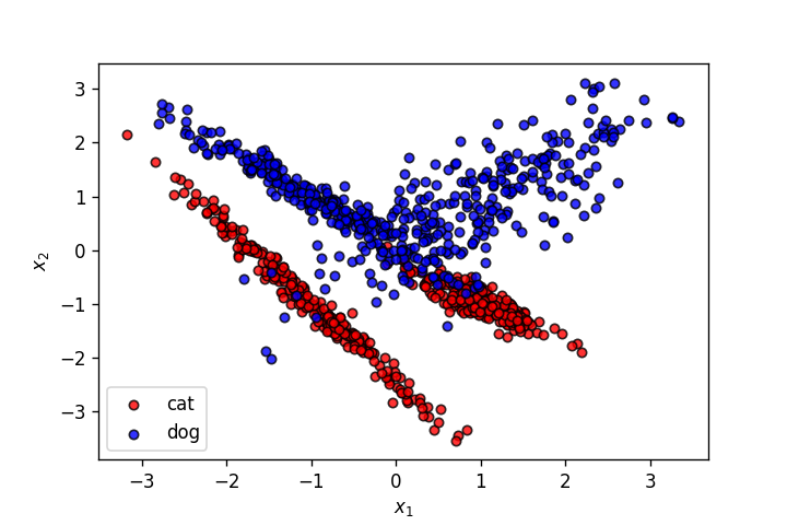
X,y = make_classification(n_samples=1000, n_features=2, n_informative=2,
                    n_redundant=0, n_repeated=0, n_classes=2, n_clusters_per_class=2,
                          class_sep=1.,
                   flip_y=0,weights=[0.5,0.5], random_state=902)
fig = plt.figure(dpi=120)
plot_points(X,y,alpha=.8)
plt.savefig('2.png')
np.random.seed(30)
nn = MLPNeuralNet3Layers(2, 3, 2, 1)

anim = create_decision_boundary_anim(nn,X,y,\
                                     epochs=600,dpi=100,\
                                     learn_rate=1e-2,snap_every=25,\
                                     print_error=True,
                                     num_cols=3)
plt.close()
HTML(anim.to_html5_video())

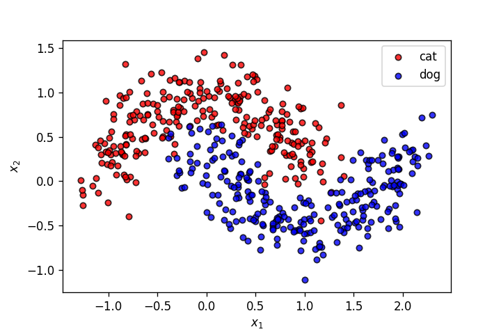
X,y = make_moons(n_samples=500, shuffle=True, noise=.2, random_state=0)
fig = plt.figure(dpi=120)
plot_points(X,y,alpha=.8)
plt.savefig('3.png')
np.random.seed(30)
nn = MLPNeuralNet3Layers(2, 3, 2, 1)

anim = create_decision_boundary_anim(nn,X,y,\
                                     epochs=300,dpi=100,\
                                     learn_rate=5e-2,snap_every=10,\
                                     print_error=True,
                                     num_cols=3)
plt.close()
HTML(anim.to_html5_video())

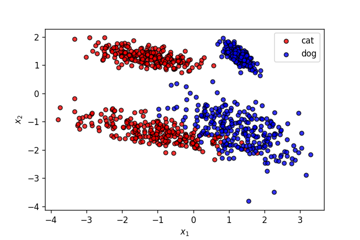
X,y = make_classification(n_samples=1000, n_features=2, n_informative=2,
                    n_redundant=0, n_repeated=0, n_classes=2, n_clusters_per_class=2,
                          class_sep=1.3,
                   flip_y=0,weights=[0.5,0.5], random_state=910)

fig = plt.figure(dpi=120)
plot_points(X,y,alpha=.8)
plt.savefig('4.png')
np.random.seed(30)
nn = MLPNeuralNet3Layers(2, 3, 2, 1)

anim = create_decision_boundary_anim(nn,X,y,\
                                     epochs=450,dpi=100,\
                                     learn_rate=5e-3,snap_every=10,\
                                     print_error=True,\
                                     num_cols=3)
plt.close()
HTML(anim.to_html5_video())

This exercise was geared more towards implementation than theory, but served as a good deep dive into understanding why adding layers to neural networks works.