This is the fourth post in this series on the basics of Machine Learning. These posts are intended to serve as companion pieces to this zine on binary classification. In the last one, we learnt how adding hidden layers to a Multilayer Perceptron helps it learn increasingly complex decision boundaries. The MLPs used till now made use of the sigmoid function as the activation function. In this post, we’ll move our focus to a much simpler kind of activation function: The Rectifier.
The rectifier was first demonstrated as a better activation function for training deep neural networks — as compared to sigmoid or hyperbolic tangent — by Xavier Glorot, Antoine Bordes, and Yoshua Bengio.
A unit employing the rectifier is called a rectified linear unit (ReLU).
ReLU, what is it?
Despite having a seemingly intimidating title, the ReLU does a very simple operation — it simply calculates the maximum of $0$ and the input. That is,
$$ \large ReLU(x) = max(0,x)$$
Or, in much simpler words: replace negatives with zeros. In fact, the inspiration for the title of this post comes from this tweet from Jeremy Howard:
1. Multiply things together
— Jeremy Howard (@jeremyphoward) March 1, 2019
2. Add them up
3. Replaces negatives with zeros
4. Return to step 1, a hundred times https://t.co/e0kwc8arjQ
import numpy as np
import matplotlib.pyplot as plt
def relu(x):
    return np.maximum(x, 0., None)
Let’s test the relu implementation on a test tensor.
test_tensor = np.array([[3,0,-4],[-4,4,1]])
test_tensor
array([[ 3,  0, -4],
       [-4,  4,  1]])
relu(test_tensor)
array([[3., 0., 0.],
       [0., 4., 1.]])
As expected, the negative values have been replaced with $0$. Let’s plot the graphs of the sigmoid and the rectifier function.
def sigmoid(x):
    return (1/(1+np.exp(-x)))
fig,axes = plt.subplots(1,2,figsize=(6,3),dpi=120)
x = np.linspace(-10,10,200)

for ax in axes.flat:
    ax.axhline(y=0, color='k')
    ax.axvline(x=0, color='k')
    ax.grid(True)

axes[0].plot(x, sigmoid(x))
axes[0].set_title('Sigmoid')

axes[1].plot(x, relu(x))
axes[1].set_xlim([-10, 10])
axes[1].set_title('ReLU')

plt.savefig('sig-vs-relu.png')
plt.show()
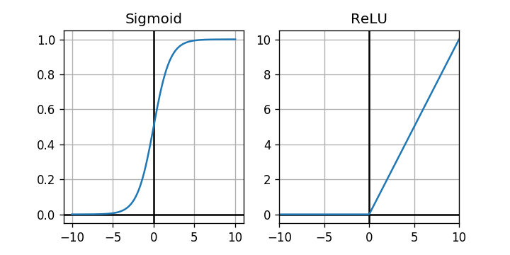
The rectifier looks like a much simpler activation function. Let’s see if it has any impact on training performance.
Setup
!apt-get -y update
!apt-get -q install imagemagick
!pip install -q celluloid
from sklearn.datasets import make_classification, make_circles, make_moons, make_blobs,make_checkerboard
import pandas as pd
from IPython.display import HTML,clear_output
import pickle
from math import ceil
from matplotlib.offsetbox import AnchoredText
from celluloid import Camera
def plot_points(X, y, alpha=None):
    dogs = X[np.argwhere(y==1)]
    cats = X[np.argwhere(y==0)]
    plt.scatter([s[0][0] for s in cats], [s[0][1] for s in cats], s = 25, \
                color = 'red', edgecolor = 'k', label='cat', alpha=alpha)
    plt.scatter([s[0][0] for s in dogs], [s[0][1] for s in dogs], s = 25, \
                color = 'blue', edgecolor = 'k', label='dog', alpha=alpha)
    plt.xlabel('$x_1$')
    plt.ylabel('$x_2$')
    plt.legend()
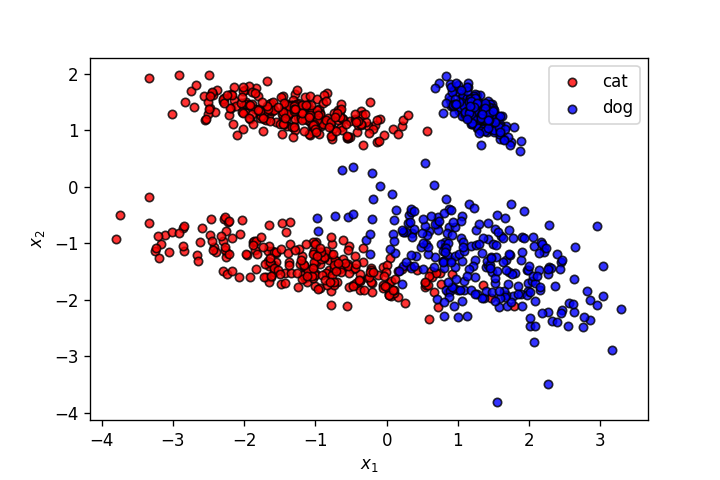
Let’s use the dataset from the last post.
!wget -q https://gist.githubusercontent.com/dhth/fcd27938c26dbc6124c1c70646a52cfc/raw/2fabb32c1008afefeaf006fcf7602638de0c8699/exor_dataset.csv
data = pd.read_csv('exor_dataset.csv', header=None)

X = np.array(data[[0,1]])
y = np.array(data[2]).astype(int)
plot_points(X,y)
plt.xlim(X[:,0].min()-0.5,X[:,0].max()+0.5)
plt.ylim(X[:,1].min()-0.5,X[:,1].max()+0.5)

plt.show()
def display_linear_boundary(ax, m, b, x_1_lims,x_2_lims,color='g--',label=None,linewidth=3.):
    ax.set_xlim(x_1_lims)
    ax.set_ylim(x_2_lims)
    x = np.arange(-10, 10, 0.1)
    ax.plot(x, m*x+b, color, label=label,linewidth=linewidth)
    ax.set_yticklabels([])
    ax.set_xticklabels([])
    return ax
def plot_points_on_ax(ax,X, y,alpha):
    dogs = X[np.argwhere(y==1)]
    cats = X[np.argwhere(y==0)]
    ax.scatter([s[0][0] for s in cats], [s[0][1] for s in cats], s = 25, \
               color = 'red', edgecolor = 'k', label='cats',alpha=alpha)
    ax.scatter([s[0][0] for s in dogs], [s[0][1] for s in dogs], s = 25, \
               color = 'blue', edgecolor = 'k', label='dogs',alpha=alpha)
    return ax
Feedforward
input_x = X[0,:].reshape(1,-1)
output_y = y[0].reshape(1,-1)
input_x.shape, output_y.shape
((1, 2), (1, 1))
N_input = 2
N_hidden_1 = 2
N_hidden_2 = 4
N_output = 1
This time we’ll initialize the weights in a different way. We’ll randomly select values from a normal distribution and then multipy them by the factor: $$ \large \sqrt{\frac{2}{\text{outputTensor.shape[1]}}} $$
I’ll get into the reasoning behind this kind of initialization — called Xavier initialisation — in an upcoming post. More details about this approach can be read here and here.
weights_input_to_hidden_1 = np.random.randn(N_input, N_hidden_1)*np.sqrt(2/N_hidden_1)
weights_hidden_1_to_hidden_2 = np.random.randn(N_hidden_1, N_hidden_2)*np.sqrt(2/N_hidden_2)
weights_hidden_2_to_output = np.random.randn(N_hidden_2, N_output)*np.sqrt(2/N_output)

bias_input_to_hidden_1 = np.zeros(N_hidden_1)
bias_hidden_1_to_hidden_2 = np.zeros(N_hidden_2)
bias_hidden_2_to_output = np.zeros(N_output)
hidden_layer_1_in = np.dot(input_x,weights_input_to_hidden_1) + bias_input_to_hidden_1
hidden_layer_1_in
array([[1.47147777, 0.01504609]])
hidden_layer_1_out = relu(hidden_layer_1_in)
hidden_layer_1_out
array([[1.47147777, 0.01504609]])
hidden_layer_2_in = np.dot(hidden_layer_1_out,weights_hidden_1_to_hidden_2) + bias_hidden_1_to_hidden_2
hidden_layer_2_in
array([[-0.59685335, 0.51556188, 0.36665501, 0.941473 ]])
hidden_layer_2_out = relu(hidden_layer_2_in)
hidden_layer_2_out
array([[0. , 0.51556188, 0.36665501, 0.941473 ]])
output_layer_in = np.dot(hidden_layer_2_out,weights_hidden_2_to_output) + bias_hidden_2_to_output
output_layer_in
array([[1.96296335]])
The activation for the final neuron has to be sigmoid as we need the MLP to output probabilities.
output_layer_out = sigmoid(output_layer_in)
output_layer_out
array([[0.8768533]])
Backpropagation
error = (-1)*(output_y*np.log(output_layer_out) + (1-output_y)*np.log(1-output_layer_out))
error
array([[2.09437893]])
del_y_out = (-1)*output_y/output_layer_out + (1-output_y)/(1-output_layer_out)
assert del_y_out.shape == output_layer_out.shape
del_y_out
array([[8.12039603]])
del_h_2 = del_y_out*output_layer_out*(1-output_layer_out)*weights_hidden_2_to_output.T
assert del_h_2.shape == hidden_layer_2_out.shape
del_h_2
array([[-0.44106764, 0.65044284, -1.85483439, 2.19440352]])
del_w_h_2_o = del_y_out*output_layer_out*(1-output_layer_out)*hidden_layer_2_out.T
assert del_w_h_2_o.shape == weights_hidden_2_to_output.shape
del_w_h_2_o
array([[0.        ],
       [0.45207213],
       [0.32150266],
       [0.82553371]])
A subtle implication of using ReLU can be seen here. As seen above, the input to the second hidden layer — hidden_layer_2_in — is [[-0.59685335, 0.51556188, 0.36665501, 0.941473 ]]. After passing this through ReLU, the first element of this set of activations will be replaced by $0$. As a result, partial derivative of the weight between first neuron of hidden layer 2 and the output neuron — del_w_h_2_om — will be $0$, as seen above.
del_b_2_o = (del_y_out*output_layer_out*(1-output_layer_out))[0]
assert del_b_2_o.shape == bias_hidden_2_to_output.shape
del_b_2_o
array([0.8768533])
hidden_layer_2_mask = hidden_layer_2_in >=0
del_h_1 = np.dot(del_h_2*hidden_layer_2_mask,weights_hidden_1_to_hidden_2.T)
assert del_h_1.shape == hidden_layer_1_out.shape
del_h_1
array([[1.1633982 , 0.61918386]])
del_w_h_1_h_2 = del_h_2*hidden_layer_2_mask*hidden_layer_1_out.T
assert del_w_h_1_h_2.shape == weights_hidden_1_to_hidden_2.shape
del_w_h_1_h_2
array([[-0.        ,  0.95711217, -2.72934756,  3.22901599],
       [-0.        ,  0.00978662, -0.027908  ,  0.03301719]])
del_b_h_1_h_2 = (del_h_2*hidden_layer_2_mask)[0]
assert del_b_h_1_h_2.shape == bias_hidden_1_to_hidden_2.shape
del_b_h_1_h_2
array([-0. , 0.65044284, -1.85483439, 2.19440352])
del_b_h_1_h_2.shape,(del_h_2*hidden_layer_2_mask)[0].shape
((4,), (4,))
hidden_layer_1_mask = hidden_layer_1_in >=0
del_w_i_h_1 = del_h_1*hidden_layer_1_mask*input_x.T
assert del_w_i_h_1.shape == weights_input_to_hidden_1.shape
del_w_i_h_1
array([[ 0.6237001 ,  0.3319457 ],
       [-0.72393617, -0.38529335]])
del_b_i_h_1 = (del_h_1*hidden_layer_1_mask)[0]
assert del_b_i_h_1.shape == bias_input_to_hidden_1.shape
del_b_i_h_1
array([1.1633982 , 0.61918386])
learn_rate = 1e-3
weights_hidden_2_to_output -= learn_rate*del_w_h_2_o
bias_hidden_2_to_output -= learn_rate*del_b_2_o

weights_hidden_1_to_hidden_2 -= learn_rate*del_w_h_1_h_2
bias_hidden_1_to_hidden_2 -= learn_rate*del_b_h_1_h_2

weights_input_to_hidden_1 -= learn_rate*del_w_i_h_1
bias_input_to_hidden_1 -= learn_rate*del_b_i_h_1
Putting all of this in a single class. To keep things simple, I’ve combined the feedforward and backpropagation steps in a single function. This is because in the case of ReLU, feedforward activations are needed to calculate partial derivatives during the backprop step. I’ve also added the function get_hidden_layer_outputs to get intermediate activations from the MLP.
class MLPNeuralNet3LayersReLU(object):
    def __init__(self,N_input, N_hidden_1, N_hidden_2, N_output,seed=None):

        if seed:
            np.random.seed(seed)

        self.weights_input_to_hidden_1 = np.random.randn(N_input, N_hidden_1)*np.sqrt(2/N_hidden_1)
        self.weights_hidden_1_to_hidden_2 = np.random.randn(N_hidden_1, N_hidden_2)*np.sqrt(2/N_hidden_2)
        self.weights_hidden_2_to_output = np.random.randn(N_hidden_2, N_output)*np.sqrt(2/N_output)

        self.bias_input_to_hidden_1 = np.zeros(N_hidden_1)
        self.bias_hidden_1_to_hidden_2 = np.zeros(N_hidden_2)
        self.bias_hidden_2_to_output = np.zeros(N_output)

    def feed_forward(self,input_x):
        self.hidden_layer_1_in = np.dot(input_x,self.weights_input_to_hidden_1) + self.bias_input_to_hidden_1
        self.hidden_layer_1_out = relu(self.hidden_layer_1_in)
        self.hidden_layer_2_in = np.dot(self.hidden_layer_1_out,self.weights_hidden_1_to_hidden_2) + self.bias_hidden_1_to_hidden_2
        self.hidden_layer_2_out = relu(self.hidden_layer_2_in)
        self.output_layer_in = np.dot(self.hidden_layer_2_out,self.weights_hidden_2_to_output) + self.bias_hidden_2_to_output
        self.output_layer_out = sigmoid(self.output_layer_in)

        return self.output_layer_out

    def get_hidden_layer_outputs(self,input_x):
        hidden_layer_1_in = np.dot(input_x,self.weights_input_to_hidden_1) + self.bias_input_to_hidden_1
        hidden_layer_1_out = relu(hidden_layer_1_in)
        hidden_layer_2_in = np.dot(hidden_layer_1_out,self.weights_hidden_1_to_hidden_2) + self.bias_hidden_1_to_hidden_2

        return (hidden_layer_1_in,hidden_layer_2_in)

    def feed_forward_and_back_propagate(self,input_x,output_y, learn_rate):
        self.hidden_layer_1_in = np.dot(input_x,self.weights_input_to_hidden_1) + self.bias_input_to_hidden_1
        self.hidden_layer_1_out = relu(self.hidden_layer_1_in)
        self.hidden_layer_2_in = np.dot(self.hidden_layer_1_out,self.weights_hidden_1_to_hidden_2) + self.bias_hidden_1_to_hidden_2
        self.hidden_layer_2_out = relu(self.hidden_layer_2_in)
        self.output_layer_in = np.dot(self.hidden_layer_2_out,self.weights_hidden_2_to_output) + self.bias_hidden_2_to_output
        self.output_layer_out = sigmoid(self.output_layer_in)

        error = (-1)*(output_y*np.log(self.output_layer_out) + (1-output_y)*np.log(1-self.output_layer_out))
        del_y_out = (-1)*output_y/self.output_layer_out + (1-output_y)/(1-self.output_layer_out)

        del_h_2 = del_y_out*self.output_layer_out*(1-self.output_layer_out)*self.weights_hidden_2_to_output.T
        del_w_h_2_o = del_y_out*self.output_layer_out*(1-self.output_layer_out)*self.hidden_layer_2_out.T
        del_b_2_o = (del_y_out*self.output_layer_out*(1-self.output_layer_out))[0]

        hidden_layer_2_mask = self.hidden_layer_2_in>0
        del_h_1 = np.dot(del_h_2*hidden_layer_2_mask,self.weights_hidden_1_to_hidden_2.T)

        del_w_h_1_h_2 = del_h_2*hidden_layer_2_mask*self.hidden_layer_1_out.T
        del_b_h_1_h_2 = (del_h_2*hidden_layer_2_mask)[0]

        hidden_layer_1_mask = self.hidden_layer_1_in >0
        del_w_i_h_1 = del_h_1*hidden_layer_1_mask*input_x.T
        del_b_i_h_1 = (del_h_1*hidden_layer_1_mask)[0]

        self.weights_hidden_2_to_output -= learn_rate*del_w_h_2_o
        self.bias_hidden_2_to_output -= learn_rate*del_b_2_o

        self.weights_hidden_1_to_hidden_2 -= learn_rate*del_w_h_1_h_2
        self.bias_hidden_1_to_hidden_2 -= learn_rate*del_b_h_1_h_2

        self.weights_input_to_hidden_1 -= learn_rate*del_w_i_h_1
        self.bias_input_to_hidden_1 -= learn_rate*del_b_i_h_1

        return error
Copying the MLP implementation from last post to compare it with the one using ReLU.
class MLPNeuralNet3LayersSigmoid(object):
    def __init__(self,N_input, N_hidden_1, N_hidden_2, N_output, seed=None):

        if seed:
            np.random.seed(seed)

        self.weights_input_to_hidden_1 = np.random.randn(N_input, N_hidden_1)*np.sqrt(1/N_hidden_1)
        self.weights_hidden_1_to_hidden_2 = np.random.randn(N_hidden_1, N_hidden_2)*np.sqrt(1/N_hidden_2)
        self.weights_hidden_2_to_output = np.random.randn(N_hidden_2, N_output)*np.sqrt(1/N_output)

        self.bias_input_to_hidden_1 = np.zeros(N_hidden_1)
        self.bias_hidden_1_to_hidden_2 = np.zeros(N_hidden_2)
        self.bias_hidden_2_to_output = np.zeros(N_output)

    def feed_forward(self,input_x):
        self.hidden_layer_1_in = np.dot(input_x,self.weights_input_to_hidden_1) + self.bias_input_to_hidden_1
        self.hidden_layer_1_out = sigmoid(self.hidden_layer_1_in)
        self.hidden_layer_2_in = np.dot(self.hidden_layer_1_out,self.weights_hidden_1_to_hidden_2) + self.bias_hidden_1_to_hidden_2
        self.hidden_layer_2_out = sigmoid(self.hidden_layer_2_in)
        self.output_layer_in = np.dot(self.hidden_layer_2_out,self.weights_hidden_2_to_output) + self.bias_hidden_2_to_output
        self.output_layer_out = sigmoid(self.output_layer_in)

        return self.output_layer_out

    def get_hidden_layer_outputs(self,input_x):
        self.hidden_layer_1_in = np.dot(input_x,self.weights_input_to_hidden_1) + self.bias_input_to_hidden_1
        self.hidden_layer_1_out = sigmoid(self.hidden_layer_1_in)
        self.hidden_layer_2_in = np.dot(self.hidden_layer_1_out,self.weights_hidden_1_to_hidden_2) + self.bias_hidden_1_to_hidden_2

        return (self.hidden_layer_1_in,self.hidden_layer_2_in)

    def back_propagate(self,input_x,output_y, learn_rate):
        error = (-1)*(output_y*np.log(self.output_layer_out) + (1-output_y)*np.log(1-self.output_layer_out))
        del_y_out = (-1)*output_y/self.output_layer_out + (1-output_y)/(1-self.output_layer_out)

        del_h_2 = del_y_out*self.output_layer_out*(1-self.output_layer_out)*self.weights_hidden_2_to_output.T
        del_w_h_2_o = del_y_out*self.output_layer_out*(1-self.output_layer_out)*self.hidden_layer_2_out.T
        del_b_2_o = (del_y_out*self.output_layer_out*(1-self.output_layer_out))[0]

        del_h_1 = np.dot(del_h_2*self.hidden_layer_2_out*(1-self.hidden_layer_2_out),self.weights_hidden_1_to_hidden_2.T)
        del_w_h_1_h_2 = del_h_2*self.hidden_layer_2_out*(1-self.hidden_layer_2_out)*self.hidden_layer_1_out.T
        del_b_h_1_h_2 = (del_h_2*self.hidden_layer_2_out*(1-self.hidden_layer_2_out))[0]

        del_w_i_h_1 = del_h_1*self.hidden_layer_1_out*(1-self.hidden_layer_1_out)*input_x.T
        del_b_i_h_1 = (del_h_1*self.hidden_layer_1_out*(1-self.hidden_layer_1_out))[0]

        self.weights_hidden_2_to_output -= learn_rate*del_w_h_2_o
        self.bias_hidden_2_to_output -= learn_rate*del_b_2_o

        self.weights_hidden_1_to_hidden_2 -= learn_rate*del_w_h_1_h_2
        self.bias_hidden_1_to_hidden_2 -= learn_rate*del_b_h_1_h_2

        self.weights_input_to_hidden_1 -= learn_rate*del_w_i_h_1
        self.bias_input_to_hidden_1 -= learn_rate*del_b_i_h_1

        return error
def train(nn, features, outputs, num_epochs, learn_rate, activation_type, print_error=False):

    for e in range(num_epochs):
        for input_x, output_y in zip(features, outputs):
            input_x = input_x.reshape(1,-1)
            output_y = output_y.reshape(1,-1)

            if activation_type == "sigmoid":
                output_layer_out = nn.feed_forward(input_x)

                error = nn.back_propagate(input_x,output_y,learn_rate=learn_rate)
            elif activation_type == "relu":
                error = nn.feed_forward_and_back_propagate(input_x,output_y,learn_rate=learn_rate)

        if print_error:
            if e%200==0:
                print(error[0][0])
    return nn
Comparisons in training performance
Instead of seeing the training performance of the new MLP in isolation, let’s compare it with the MLP from the last post.
def compare_sigmoid_and_relu(nn_1,nn_2,X,y,epochs=300,learn_rate=1e-3,snap_every=100,dpi=100,
                                  print_error=False,
                                  activation_types=['sigmoid','relu'],
                                  titles=['Sigmoid','ReLU']):

    nns = [nn_1,nn_2]

    hidden_layer_1_units = nn_1.weights_hidden_1_to_hidden_2.shape[0]
    hidden_layer_2_units = nn_1.weights_hidden_2_to_output.shape[0]

    num_rows = 1 + hidden_layer_1_units + hidden_layer_2_units
    num_cols = 2

    fig,axes = plt.subplots(num_rows, num_cols, figsize=(num_cols*3,num_rows*3),dpi=dpi)

    axes_list = list(axes.flat)

    for ax in axes.flat:
        ax.set_yticklabels([])
        ax.set_xticklabels([])
        ax.get_xaxis().set_visible(False)
        ax.get_yaxis().set_visible(False)

    nn_1_axes = axes_list[0::2]
    nn_2_axes = axes_list[1::2]

    nns_axes = [nn_1_axes,nn_2_axes]

    final_dec_boundary_ax = axes_list[0]

    hidden_layer_1_ax = axes_list[1:hidden_layer_1_units+1]
    hidden_layer_2_ax = axes_list[hidden_layer_1_units+1:hidden_layer_1_units+1+hidden_layer_2_units]

    camera = Camera(fig)

    h = .02

    extra_space = 0.5
    x_min, x_max = X[:, 0].min() - extra_space, X[:, 0].max() + extra_space
    y_min, y_max = X[:, 1].min() - extra_space, X[:, 1].max() + extra_space
    xx, yy = np.meshgrid(np.arange(x_min, x_max, h),
                     np.arange(y_min, y_max, h))

    for e in range(ceil(epochs/snap_every)):
        for j,nn in enumerate(nns):
            nn = train(nn,X,y,snap_every,learn_rate,activation_types[j],print_error=print_error)
            Z = (nn.feed_forward(np.c_[xx.ravel(), yy.ravel()]) >0.5).astype(int)
            Z = Z.reshape(xx.shape)
            nns_axes[j][0].contourf(xx, yy, Z, cmap=plt.cm.RdBu)

            text_box = AnchoredText(f'Epoch: {snap_every*(e+1)}', frameon=True, loc=4, pad=0.5)
            plt.setp(text_box.patch, facecolor='white', alpha=0.5)
            nns_axes[j][0].add_artist(text_box)

            Z_hidden_1, Z_hidden_2 = nn.get_hidden_layer_outputs(np.c_[xx.ravel(), yy.ravel()])
            Z_hidden_1 = (Z_hidden_1 >0.).astype(int)
            Z_hidden_2 = (Z_hidden_2 >0.).astype(int)

            for i,ax in enumerate(nns_axes[j][1:hidden_layer_1_units+1]):
                Z_ = Z_hidden_1[:,i].reshape(-1,1)
                Z_ = Z_.reshape(xx.shape)
                ax.contourf(xx, yy, Z_, cmap=plt.cm.RdBu)

            for i,ax in enumerate(nns_axes[j][hidden_layer_1_units+1:hidden_layer_1_units+1+hidden_layer_2_units]):
                Z_ = Z_hidden_2[:,i].reshape(-1,1)
                Z_ = Z_.reshape(xx.shape)
                ax.contourf(xx, yy, Z_, cmap=plt.cm.RdBu)

        camera.snap()


    for j,nn in enumerate(nns):
        nns_axes[j][0] = plot_points_on_ax(nns_axes[j][0],X, y,alpha=.6)
        nns_axes[j][0].set_title(f'NN with {titles[j]}\n\nOutput Decision Boundary')

        for i,ax in enumerate(nns_axes[j][1:hidden_layer_1_units+1]):
            ax = plot_points_on_ax(ax,X, y,alpha=.6)
            ax.set_title(f'Hidden layer 1 neuron {i+1}')

        for i,ax in enumerate(nns_axes[j][hidden_layer_1_units+1:hidden_layer_1_units+1+hidden_layer_2_units]):
            ax = plot_points_on_ax(ax,X, y,alpha=.6)
            ax.set_title(f'Hidden layer 2 neuron {i+1}')


    plt.annotate('https://dhruvs.space', xy=(1, 0), xycoords='axes fraction', fontsize=9,
                xytext=(0, -15), textcoords='offset points',
                ha='right', va='top')
    plt.tight_layout()
    animation = camera.animate()

    return animation
seed = 30
n_hidden_1 = 4
n_hidden_2 = 3

nn_1 = MLPNeuralNet3LayersSigmoid(2, n_hidden_1, n_hidden_2, 1, seed=seed)
nn_2 = MLPNeuralNet3LayersReLU(2,n_hidden_1, n_hidden_2, 1, seed=seed)

anim = compare_sigmoid_and_relu(nn_1,nn_2,X,y,\
                                     epochs=20,dpi=100,\
                                     learn_rate=1e-2,snap_every=1,\
                                     print_error=False
                                     )
plt.close()
HTML(anim.to_html5_video())

The MLP from the last post was getting this level of accuracy after 300-400 epochs, while the one using ReLU is achieving that in around 20 epochs. That’s a huge improvement in training performance.
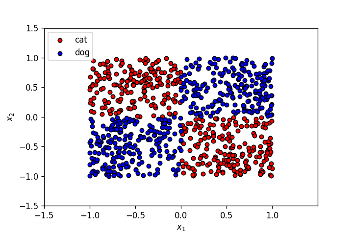
Let’s see the results on a few more datasets.
X,y = make_classification(n_samples=1000, n_features=2, n_informative=2,
                    n_redundant=0, n_repeated=0, n_classes=2, n_clusters_per_class=2,
                          class_sep=1.,
                   flip_y=0,weights=[0.5,0.5], random_state=902)

plot_points(X,y,alpha=.8)
seed = 10
n_hidden_1 = 4
n_hidden_2 = 3

nn_1 = MLPNeuralNet3LayersSigmoid(2, n_hidden_1, n_hidden_2, 1, seed=seed)
nn_2 = MLPNeuralNet3LayersReLU(2,n_hidden_1, n_hidden_2, 1, seed=seed)

anim = compare_sigmoid_and_relu(nn_1,nn_2,X,y,\
                                     epochs=15,dpi=100,\
                                     learn_rate=1e-2,snap_every=1,\
                                     print_error=False
                                     )
plt.close()
HTML(anim.to_html5_video())
HTML(anim.to_html5_video())

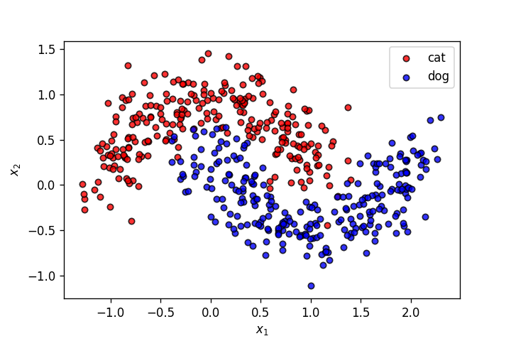
X,y = make_moons(n_samples=500, shuffle=True, noise=.2, random_state=0)

plot_points(X,y,alpha=.8)
seed = 10
n_hidden_1 = 4
n_hidden_2 = 3

nn_1 = MLPNeuralNet3LayersSigmoid(2, n_hidden_1, n_hidden_2, 1, seed=seed)
nn_2 = MLPNeuralNet3LayersReLU(2,n_hidden_1, n_hidden_2, 1, seed=seed)

anim = compare_sigmoid_and_relu(nn_1,nn_2,X,y,\
                                     epochs=50,dpi=100,\
                                     learn_rate=1e-2,snap_every=2,\
                                     print_error=False
                                     )
plt.close()
HTML(anim.to_html5_video())
HTML(anim.to_html5_video())

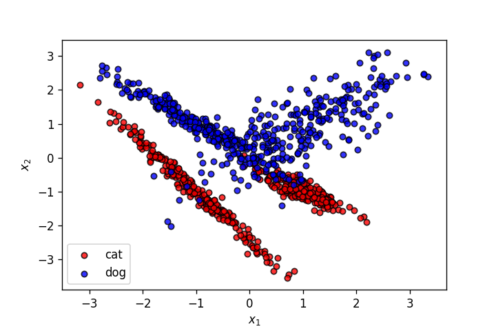
X,y = make_classification(n_samples=1000, n_features=2, n_informative=2,
                    n_redundant=0, n_repeated=0, n_classes=2, n_clusters_per_class=2,
                          class_sep=1.3,
                   flip_y=0,weights=[0.5,0.5], random_state=910)


plot_points(X,y,alpha=.8)
seed = 10
n_hidden_1 = 3
n_hidden_2 = 2

nn_1 = MLPNeuralNet3LayersSigmoid(2, n_hidden_1, n_hidden_2, 1, seed=seed)
nn_2 = MLPNeuralNet3LayersReLU(2,n_hidden_1, n_hidden_2, 1, seed=seed)

anim = compare_sigmoid_and_relu(nn_1,nn_2,X,y,\
                                     epochs=50,dpi=100,\
                                     learn_rate=1e-2,snap_every=2,\
                                     print_error=False
                                     )
plt.close()
HTML(anim.to_html5_video())
HTML(anim.to_html5_video())

As seen above, in every case the MLP using ReLU as activation is learning to segment the training dataset way faster, as compared to the MLP using sigmoid.