I just started Udacity’s Intro to Self Driving Cars Nanodegree and the very first thing the instructors teach in it is Bayes’ theorem. I read about it in school, but now’s the time for me to really get into it, hence this summary note.
Bayes’ theorem gives a mathematical way to correct predictions about probability of an event, and move from prior belief to something more and more probable.
The intuition behind application of Bayes’ theorem in probabilistic inference can be put as follows:
Given an initial prediction, if we gather additional related data, data that the initial prediction depends upon, we can improve that prediction.
Example
Let’s say the probability of people having the mutant X-gene, P(X) is $0.01$. There’s a test to detect the gene which results in a positive or negative outcome. In case of people who actually have the X-gene this test results positive $90%$ of the time. In the case of people who don’t have the X-gene, this test results negative $90%$ of the time.
The question to answer is:
Given that the test comes out positive for a person, what is the probability of that person being a mutant?
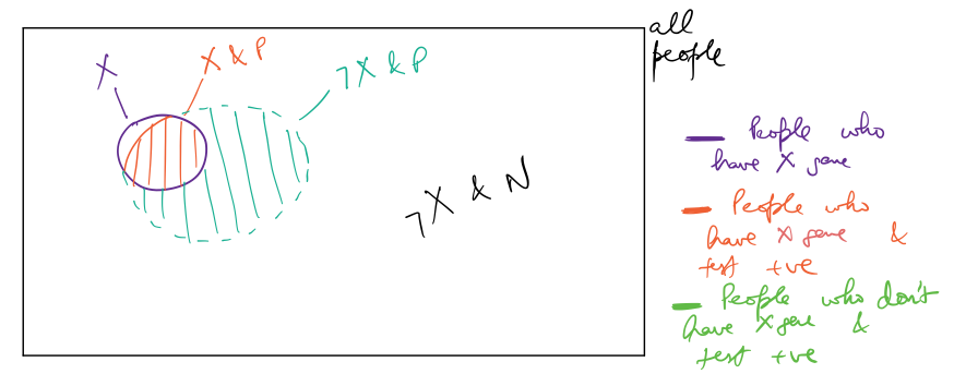
Let’s try to visualize this scenario. In the figure below the box represents all people. Inside the box, the purple circle represents people who actually have the X-gene, ie, $1%$ of all people. The red highlighted area is the $90%$ of the purple circle, and represents people who actually have the X-gene and test positive. The green highlighted is $10%$ of the area of the box (ie, $10%$ of all people), and represents people who don’t have the X-gene and test positive.
Essence of Bayes’ Rule
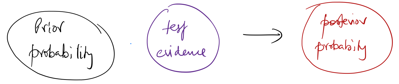
We start with a prior probability, and incorporate test evidence, and arrive at the posterior probability.
Bayes’ rule states:
$$ \large P(X\mid Pos) = \frac{P(Pos\mid X) \cdot P(X) }{P(Pos)} $$
which is also equal to
$$ \large P(X\mid Pos) = \frac{P(Pos,X)}{P(Pos)} $$
where $P(Pos,X)$ is the joint probability of a person having the X-gene and also testing positive.
From given data, $P(Pos\mid X)$ is $0.9$, $P(X)$ is $0.01$.
Total probability of testing positive, ie, $P(Pos)$, is the sum of joint probabilities of testing positive and having the X-gene, and testing positive and not having the X-gene. That is:
$$ \large P(Pos) = P(Pos\mid X) \cdot P(X) + P(Pos\mid \neg X) \cdot P(\neg X)$$
So, finally:
$$ \large P(X\mid Pos) = \frac{P(Pos\mid X) \cdot P(X) }{P(Pos\mid X) \cdot P(X) + P(Pos\mid \neg X) \cdot P(\neg X)} $$
Putting in the values, it turns out to be:
$$ \large P(X\mid Pos) = \frac{0.9 \cdot 0.01 }{0.9 \cdot 0.01 + 0.1 \cdot 0.99} = 0.0833$$
Putting all of this process in a flowchart:
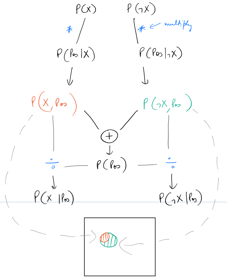
As seen above the two joint probabilities represent the corresponding color coded areas in the diagram shown before.