This post is first in a series on object detection. The succeeding posts can be found here, here, and here.
One of the primary takeaways for me after learning the basics of object detection was that the very backbone of the convnet architecture used for classification can also be utilised for localization. Intuitively, it does make sense, as convnets tend to preserve spatial information present in the input images. I saw some of that in action (detailed here and here) while generating localization maps from activations of the last convolutional layer of a Resnet-34, which was my first realization that a convnet really does take into consideration the spatial arrangement of pixels while coming up with a class score.
Without knowing that bit of information, object detection does seem like a hard problem to solve! Accurate detection of multiple kinds of similar looking objects is a tough one to solve even today, but starting out with a basic detector is not overly complex. Or atleast, the concepts behind it are fairly straightforward (I get to say that thanks to the hard work of numerous researchers).
Let’s write a detector for objects in the Pascal VOC dataset.
The approach used below is based on learnings from fastai’s Deep Learning MOOC (Part 2).
Setup
%matplotlib inline
%reload_ext autoreload
%autoreload 2
!pip install -q fastai==0.7.0 torchtext==0.2.3
!wget -qq http://pjreddie.com/media/files/VOCtrainval_06-Nov-2007.tar
!tar -xf VOCtrainval_06-Nov-2007.tar
!wget -qq https://storage.googleapis.com/coco-dataset/external/PASCAL_VOC.zip
!unzip -q PASCAL_VOC.zip
!mkdir -p data/pascal
!mv PASCAL_VOC/* data/pascal
!mv VOCdevkit data/pascal
DRIVE_BASE_PATH = "/content/gdrive/My\ Drive/Colab\ Notebooks/"
from fastai.conv_learner import *
from fastai.dataset import *
from pathlib import Path
import json
from PIL import ImageDraw, ImageFont
from matplotlib import patches, patheffects
Fetching Pascal VOC dataset and annotations.
PATH = Path('data/pascal')
list(PATH.iterdir())
[PosixPath('data/pascal/pascal_val2007.json'),
 PosixPath('data/pascal/VOCdevkit'),
 PosixPath('data/pascal/pascal_val2012.json'),
 PosixPath('data/pascal/pascal_train2007.json'),
 PosixPath('data/pascal/pascal_train2012.json'),
 PosixPath('data/pascal/pascal_test2007.json')]
trn_j = json.load((PATH/'pascal_train2007.json').open())
trn_j.keys()
dict_keys(['images', 'type', 'annotations', 'categories'])
IMAGES,ANNOTATIONS,CATEGORIES = ['images', 'annotations', 'categories']
trn_j[ANNOTATIONS][:2]
[{'area': 34104,
  'bbox': [155, 96, 196, 174],
  'category_id': 7,
  'id': 1,
  'ignore': 0,
  'image_id': 12,
  'iscrowd': 0,
  'segmentation': [[155, 96, 155, 270, 351, 270, 351, 96]]},
 {'area': 13110,
  'bbox': [184, 61, 95, 138],
  'category_id': 15,
  'id': 2,
  'ignore': 0,
  'image_id': 17,
  'iscrowd': 0,
  'segmentation': [[184, 61, 184, 199, 279, 199, 279, 61]]}]
trn_j[CATEGORIES][:4]
[{'id': 1, 'name': 'aeroplane', 'supercategory': 'none'},
 {'id': 2, 'name': 'bicycle', 'supercategory': 'none'},
 {'id': 3, 'name': 'bird', 'supercategory': 'none'},
 {'id': 4, 'name': 'boat', 'supercategory': 'none'}]
FILE_NAME,ID,IMG_ID,CAT_ID,BBOX = 'file_name','id','image_id','category_id','bbox'

cats = {o[ID]:o['name'] for o in trn_j[CATEGORIES]}
trn_fns = {o[ID]:o[FILE_NAME] for o in trn_j[IMAGES]}
trn_ids = [o[ID] for o in trn_j[IMAGES]]
list((PATH/'VOCdevkit'/'VOC2007').iterdir())
[PosixPath('data/pascal/VOCdevkit/VOC2007/SegmentationObject'),
 PosixPath('data/pascal/VOCdevkit/VOC2007/ImageSets'),
 PosixPath('data/pascal/VOCdevkit/VOC2007/JPEGImages'),
 PosixPath('data/pascal/VOCdevkit/VOC2007/Annotations'),
 PosixPath('data/pascal/VOCdevkit/VOC2007/SegmentationClass')]
JPEGS = 'VOCdevkit/VOC2007/JPEGImages'
IMG_PATH = PATH/JPEGS
What do we have here? :
- A directory of images
- JSON files with annotations for each image. Annotations contain bounding boxes for all objects (eg. car, person) in the training set, ie, each object is mapped to a category, and an image.
How do we make this data easier to use for training a network?
- Create a python dictionary which maps an image id to a list of annotations for all objects in that image, ie, list of tuples each representing
(ndarray of bounding box, category_id). - We convert VOC’s height/width into top-left/bottom-right coordinates, and switch x/y coords to be consistent with numpy.
def hw_bb(bb): return np.array([bb[1], bb[0], bb[3]+bb[1]-1, bb[2]+bb[0]-1])

trn_anno = collections.defaultdict(lambda:[])
for o in trn_j[ANNOTATIONS]:
    if not o['ignore']:
        bb = o[BBOX]
        bb = hw_bb(bb)
        trn_anno[o[IMG_ID]].append((bb,o[CAT_ID]))
Let’s check out one of the images (randomly choosing image with id 1237).
def show_img(im, figsize=None, ax=None):
    if not ax: fig,ax = plt.subplots(figsize=figsize)
    ax.imshow(im)
    ax.get_xaxis().set_visible(False)
    ax.get_yaxis().set_visible(False)
    return ax
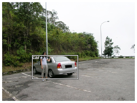
show_img(open_image(IMG_PATH/trn_fns[1237]),figsize=(10,6));
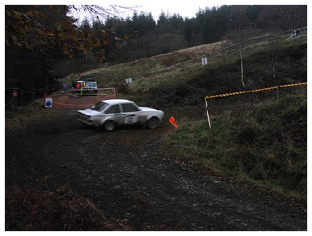
It’s a car. Let’s see how this is represented in the annotations.
im_a = trn_anno[1237]; im_a
[(array([155, 114, 212, 265]), 7)]
cats[7]
'car'
As expected, it’s an array of tuples containing bounding box and a category. Let’s check out an image containing two objects.
show_img(open_image(IMG_PATH/trn_fns[4779]),figsize=(10,6));
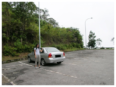
trn_anno[17]
[(array([ 61, 184, 198, 278]), 15), (array([ 77, 89, 335, 402]), 13)]
cats[15],cats[13]
('person', 'horse')
As expected, we’ve got annotations for each object present in the image. Now let’s plot these bounding boxes on these images. Since matplotlib’s patch takes in bounding boxes in the format of height-width we’ll use bb_hw to convert top-left/bottom-right coordinates into the appropriate format.
def bb_hw(a): return np.array([a[1],a[0],a[3]-a[1]+1,a[2]-a[0]+1])
One of the many simple-but-effective techniques I learnt from fastai’s MOOC is the following approach for plotting elements on an image: Making text and patches visible regardless of background by adding a boundary with a different color.
def draw_outline(o, lw, foreground_color='black'):
    o.set_path_effects([patheffects.Stroke(
        linewidth=lw, foreground=foreground_color), patheffects.Normal()])

def draw_rect(ax, b, color="white", foreground_color='black'):
    patch = ax.add_patch(patches.Rectangle(b[:2], *b[-2:], fill=False, edgecolor=color, lw=2))
    draw_outline(patch, 4, foreground_color)

def draw_text(ax, xy, txt, sz=14):
    text = ax.text(*xy, txt,
        verticalalignment='top', color='white', fontsize=sz, weight='bold')
    draw_outline(text, 1)
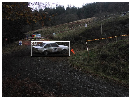
im = open_image(IMG_PATH/trn_fns[1237])
ax = show_img(im,figsize=(10,6))
b = bb_hw(trn_anno[1237][0][0])
draw_rect(ax, b)
draw_text(ax, b[:2], cats[trn_anno[12][0][1]])
def draw_im(im, ann):
#     ax = show_img(im, figsize=(16,8))
    ax = show_img(im,figsize=(10,6))
    for b,c in ann:
        b = bb_hw(b)
        draw_rect(ax, b)
        draw_text(ax, b[:2], cats[c], sz=16)
def draw_idx(i):
    im_a = trn_anno[i]
    im = open_image(IMG_PATH/trn_fns[i])
    draw_im(im, im_a)
draw_idx(4779)
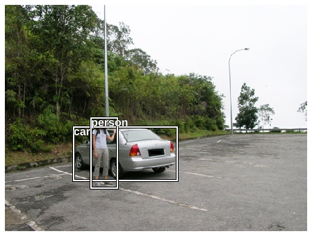
Alright! We can now visually see annotations in the training data.
Let’s think of multiple-object detection in an iterative manner. Let’s begin with single object detection:
- We’ll start by classifying the largest object in an image.
- Then we’ll localize this largest object, ie, output a bounding box for it.
- Finally, we’ll do both at the same time, ie, answer the question “What’s the largest object in the image and where is it?”
Stage 1: Largest item classifier
We only need annotations for the largest object per image ie, bounding box having largest area.
for a,b in trn_anno[4779]:
    print(f'bb for {cats[b]}: {a}')
    print(f'\tarea = {(a[-2:]-a[:2])[0]} * {(a[-2:]-a[:2])[1]} = {np.product(a[-2:]-a[:2])}')
bb for car: [202 113 290 283]
	area = 88 * 170 = 14960
bb for person: [187 142 303 184]
	area = 116 * 42 = 4872
def get_lrg(b):
    if not b: raise Exception()
    b = sorted(b, key=lambda x: np.product(x[0][-2:]-x[0][:2]), reverse=True)
    return b[0]
trn_lrg_anno = {a: get_lrg(b) for a,b in trn_anno.items()}
b,c = trn_lrg_anno[4779]
b = bb_hw(b)
ax = show_img(open_image(IMG_PATH/trn_fns[4779]),figsize=(10,6))
draw_rect(ax, b)
draw_text(ax, b[:2], cats[c], sz=16)
We’ve filtered the annotations from the original dataset to only contain one object per image. Let’s build a simple convnet classifier for this dataset. I won’t focus too much on fastai specific techniques for building neural networks as it’s not the primary motivation behind this exercise.
(PATH/'tmp').mkdir(exist_ok=True)
CSV = PATH/'tmp/lrg.csv'
df = pd.DataFrame({'fn': [trn_fns[o] for o in trn_ids],
    'cat': [cats[trn_lrg_anno[o][1]] for o in trn_ids]}, columns=['fn','cat'])
df.to_csv(CSV, index=False)
f_model = resnet34
sz=224
bs=64
tfms1 = tfms_from_model(f_model, sz, aug_tfms=transforms_side_on, crop_type=CropType.NO)
md1 = ImageClassifierData.from_csv(PATH, JPEGS, CSV, tfms=tfms1, bs=bs)
learn = ConvLearner.pretrained(f_model, md1, metrics=[accuracy])
learn.opt_fn = optim.Adam
lr = 2e-2
learn.fit(lr, 1, cycle_len=1)
lrs = np.array([lr/1000,lr/100,lr])
learn.freeze_to(-2)
learn.fit(lrs/5, 1, cycle_len=1)
learn.unfreeze()
learn.fit(lrs/5, 1, cycle_len=2)
Accuracy isn’t improving much beyond 80% since VOC isn’t ideal for single object classification as many images have multiple different objects. Let’s see the network’s predictions on a validation batch.
learn.save('clas_one')
!cp {PATH}/models/clas_one.h5 {DRIVE_BASE_PATH}saved_models/fai_part_2/lec_8/
!cp {DRIVE_BASE_PATH}saved_models/fai_part_2/lec_8/clas_one.h5 {PATH}/models/
learn.load('clas_one')
def show_validation_batch_lrg_classifier(batch_num):
val_iter = iter(md1.val_dl)
for i in range(batch_num):
next(val_iter)
x,y = next(val_iter)
probs = F.softmax(predict_batch(learn.model, x), -1)
x,preds = to_np(x),to_np(probs)
preds = np.argmax(preds, -1)
fig, axes = plt.subplots(3, 4, figsize=(10, 6))
for i,ax in enumerate(axes.flat):
ima=md1.val_ds.denorm(x)[i]
b = md1.classes[preds[i]]
ax = show_img(ima, ax=ax)
act = md1.classes[y[i]]
if not act==b:
ax.set_title(f'act: {md.classes[y[i]]} | pred: {b}')
else:
ax.set_title(f'correct: {b}')
plt.tight_layout()
fig_name = f'plots-1-batch-{batch_num}.png'
plt.savefig(fig_name)
print(f'')
plt.close(fig)
show_validation_batch_lrg_classifier(1)
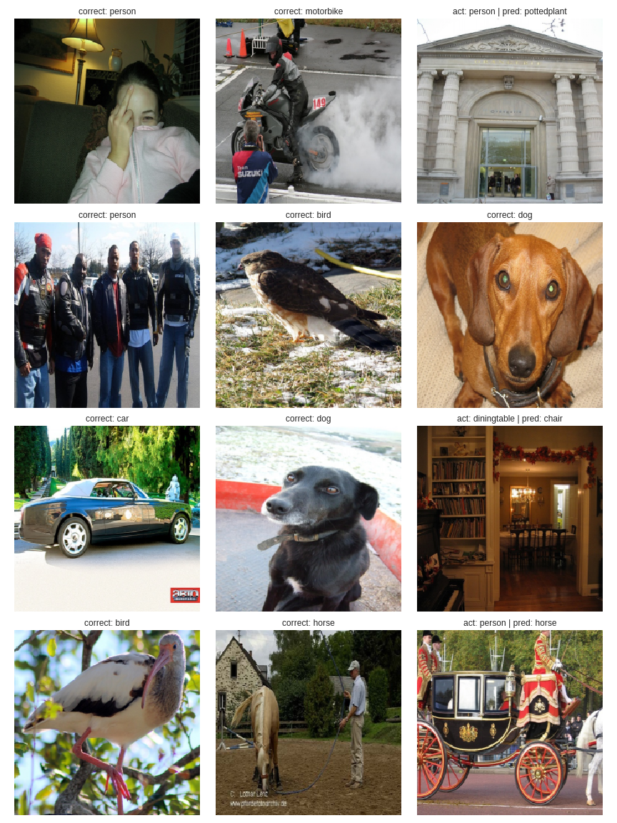
show_validation_batch_lrg_classifier(2)
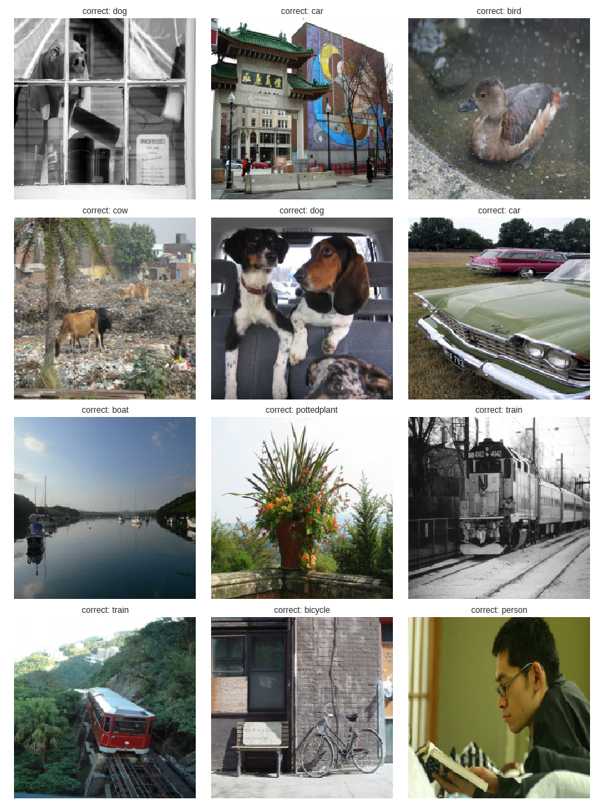
show_validation_batch_lrg_classifier(3)
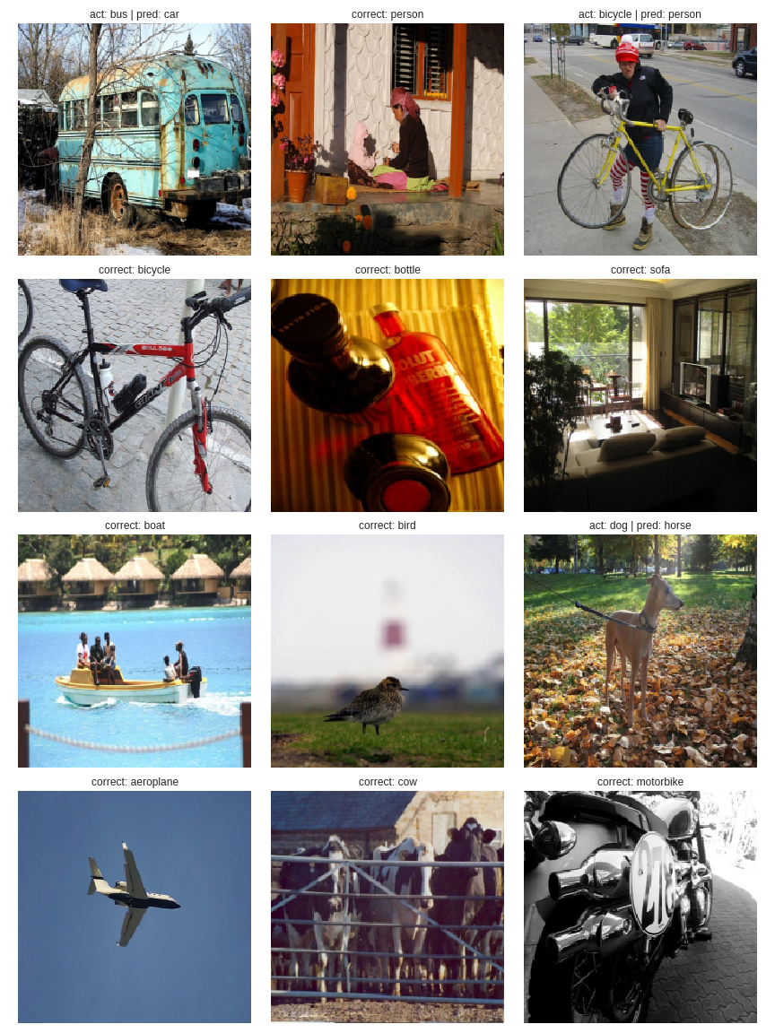
It’s doing a pretty good job of classifying the largest object! As expected, it’s mostly mis-classifying when images have multiple objects.
Stage 2: Localization only
Let’s move on to stage 2 of single-object detection, ie, localizing the largest object in an image.
What do we need to achieve this?
We need 2 coordinates corresponding to top-left and bottom-right corners of the bounding box for that object, ie, we need the network to output 4 numbers. This is a multiple column regression problem instead of a classification one.
Loss function
We can directly compare the L1 distance between the activations from the network and the training x-y coordinates.
BB_CSV = PATH/'tmp/bb.csv'
bb = np.array([trn_lrg_anno[o][0] for o in trn_ids])
bbs = [' '.join(str(p) for p in o) for o in bb]

df = pd.DataFrame({'fn': [trn_fns[o] for o in trn_ids], 'bbox': bbs}, columns=['fn','bbox'])
df.to_csv(BB_CSV, index=False)
f_model=resnet34
sz=224
bs=64
Before we create the model, we need to handle some data augmentation specific intricacies. We want the bounding box coordinates to be appropriately manipulated when fastai augments the images during training.
tfm_y = TfmType.COORD
augs2 = [RandomFlip(tfm_y=tfm_y),
        RandomRotate(3, p=0.5, tfm_y=tfm_y),
        RandomLighting(0.05,0.05, tfm_y=tfm_y)]

tfms2 = tfms_from_model(f_model, sz, crop_type=CropType.NO, tfm_y=tfm_y, aug_tfms=augs2)
md2 = ImageClassifierData.from_csv(PATH, JPEGS, BB_CSV, tfms=tfms2, bs=bs, continuous=True)
Now we’ll modify the “head” of the network as per our requirement for localization. That is, instead of using the default final layers of a ResNet-34 (average pooling and fully connected layers), we’ll first flatten the output of the final Batch Norm layer, and add a simple Linear layer with 4 units. Also, we don’t want to use any sort of activation to the final outputs since we’re comparing L1 distances with X-Y coordinates.
The final Batch-Norm layer’s output is of shape (-1,512,7,7), so we need 512*7*7 dimensional input to the Linear layer.
head_reg4 = nn.Sequential(Flatten(), nn.Linear(512*7*7,4))

learn2 = ConvLearner.pretrained(f_model, md2, custom_head=head_reg4)
learn2.opt_fn = optim.Adam
learn2.crit = nn.L1Loss()
lr = 2e-3
learn2.fit(lr, 2, cycle_len=1, cycle_mult=2)
lrs = np.array([lr/100,lr/10,lr])
learn2.freeze_to(-2)
learn2.fit(lrs, 2, cycle_len=1, cycle_mult=2)
learn2.freeze_to(-3)
learn2.fit(lrs, 1, cycle_len=2)
Getting an MSE loss of around 20, which is pretty good for this simple network. Let’s see validation results.
learn2.save('reg4')
!cp {PATH}/models/reg4.h5 {DRIVE_BASE_PATH}saved_models/fai_part_2/lec_8/
!cp {DRIVE_BASE_PATH}saved_models/fai_part_2/lec_8/reg4.h5 {PATH}/models/
learn2.load('reg4')
def show_validation_batch(batch_num):
val_iter = iter(md2.val_dl)
for i in range(batch_num):
next(val_iter)
x,y = next(val_iter)
m = learn2.model.eval()
preds = to_np(m(VV(x)))
fig, axes = plt.subplots(3, 4, figsize=(10, 8))
for i,ax in enumerate(axes.flat):
ima=md2.val_ds.denorm(to_np(x))[i]
b = bb_hw(preds[i])
ax = show_img(ima, ax=ax)
draw_rect(ax, b)
draw_rect(ax, bb_hw(y[i]),color="red")
plt.tight_layout()
fig_name = f'plots-2-batch-{batch_num}.png'
plt.savefig(fig_name)
print(f'')
plt.close(fig)
Red bounded boxes are the ground truth.
show_validation_batch(1)
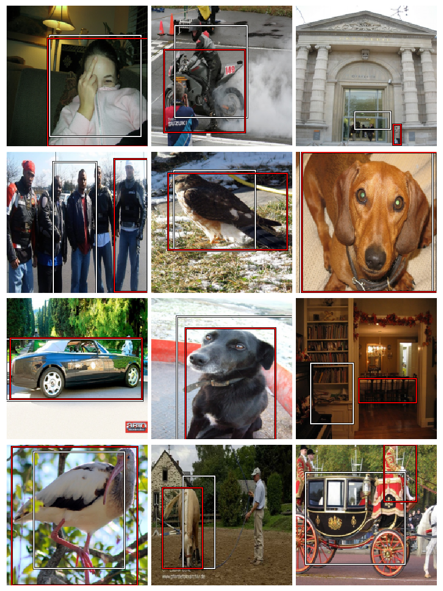
show_validation_batch(2)
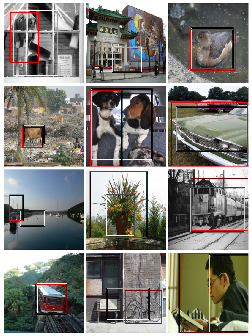
show_validation_batch(3)
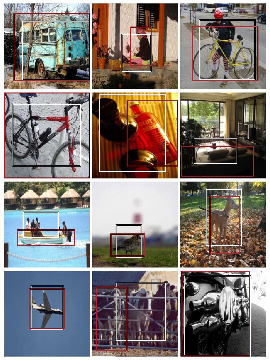
This simple network seems to be doing reasonably well on images containing a single object. It’s not doing so good with images containing multiple objects, and is doing particulary bad when the image contains very small objects.
I’m still curious as to see if the two architectures put different weightages to pixel arrangements based on the final layers. Let’s plot heat-maps for the validation batch using forward pass activations. To read more on the technique used see here.
m1 = learn.model.eval();
m2 = learn2.model.eval();
def save_outputs_classifier(self, input, output):
    outputs_classifier.append(output.data)

def save_outputs_localizer(self, input, output):
    outputs_localizer.append(output.data)
last_conv_hook_handle_cl = m1[7].register_forward_hook(save_outputs_classifier)
last_conv_hook_handle_lo = m2[7].register_forward_hook(save_outputs_localizer)
def show_validation_batch_with_heat_maps(batch_num, num_rows=5):
val_iter1 = iter(md1.val_dl)
for i in range(batch_num):
next(val_iter1)
x1,y1 = next(val_iter1)
# getting predictions from classifier
probs1 = F.softmax(predict_batch(m1, x1), -1)
preds1 = to_np(probs1)
preds1 = np.argmax(preds1, -1)
x1 = to_np(x1)
val_iter2 = iter(md2.val_dl)
for i in range(batch_num):
next(val_iter2)
x2,y2 = next(val_iter2)
# getting predictions from localizer
preds2 = to_np(m2(VV(x2)))
x2 = to_np(x2)
# activations from classifier
acts1 = outputs_classifier[0].cpu()
avg_acts1 = acts1.mean(1)
# activations from localizer
acts2 = outputs_localizer[0].cpu()
avg_acts2 = acts2.mean(1)
fig, axes = plt.subplots(num_rows, 3, figsize=(6, num_rows*2))
i = 0
for j in range(x1.shape[0]):
if i==num_rows:
break
ima=md1.val_ds.denorm(x1)[j]
b = md1.classes[preds1[j]]
act = md1.classes[y1[j]]
if not act==b: # only plotting images where classifier is incorrect
# 1st column
axes[i,0] = show_img(ima, ax=axes[i,0])
# 2nd column
axes[i,1] = show_img(ima, ax=axes[i,1])
axes[i,1].imshow(avg_acts1[j], alpha=0.6, extent=(0,224,224,0),
interpolation='bilinear', cmap='magma');
act = md1.classes[y1[j]]
axes[i,1].set_title(f'act: {md1.classes[y1[j]]} | pred: {b}')
# 3rd column
ima=md2.val_ds.denorm(x2)[j]
b = bb_hw(preds2[j])
axes[i,2] = show_img(ima, ax=axes[i,2])
axes[i,2].imshow(avg_acts2[j], alpha=0.6, extent=(0,224,224,0),
interpolation='bilinear', cmap='magma');
draw_rect(axes[i,2], b)
draw_rect(axes[i,2], bb_hw(y2[j]),color="red")
i+=1
plt.tight_layout()
fig_name = f'plots-heat-maps-batch-{batch_num}.png'
plt.savefig(fig_name)
print(f'')
plt.close(fig)
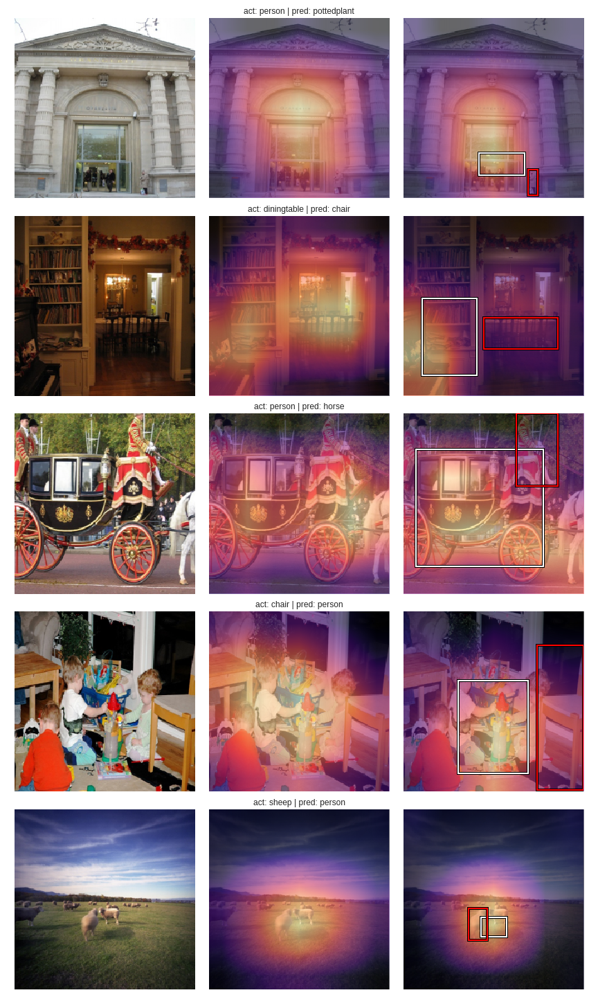
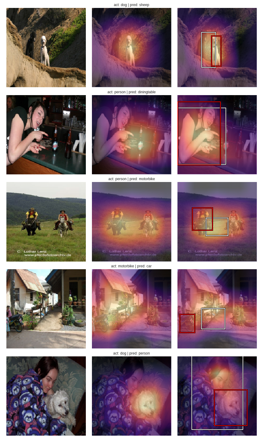
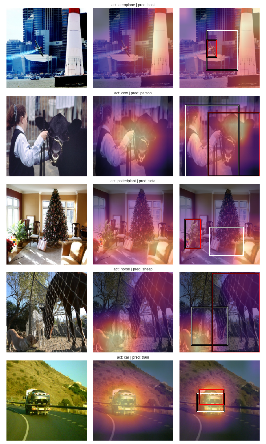
The plot shows original image, classifier heat-maps, and localizer heatmaps in 1st, 2nd, and 3rd columns respectively.
outputs_classifier = []
outputs_localizer = []
show_validation_batch_with_heat_maps(1,5)
outputs_classifier = []
outputs_localizer = []
show_validation_batch_with_heat_maps(2,5)
outputs_classifier = []
outputs_localizer = []
show_validation_batch_with_heat_maps(4,5)
outputs_classifier = []
outputs_localizer = []
show_validation_batch_with_heat_maps(5,5)
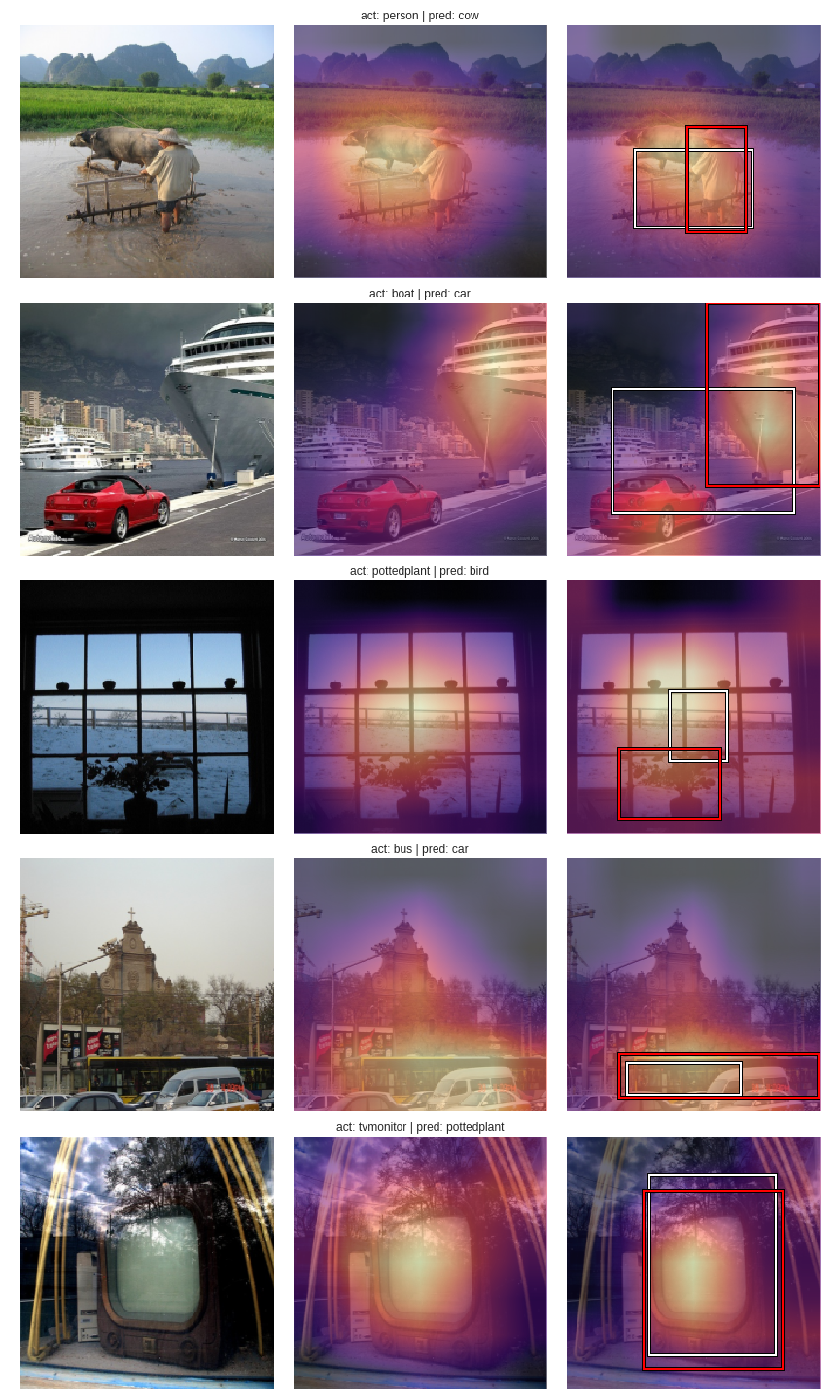
For the most part, the heat-maps seem to be concentrated in same regions for both approaches. Since the classifier and localizer are two separate models, we can’t correlate the position of a bounding box with a class. One insight I can gather from the heat-maps from the localizer is that when these maps are sparse (ie, not concentrated on a particular region), it comes up with a seemingly random bounding box mostly situated at the center of the image.
The finding from this exercise is that we can switch from classification to localization by simply changing the final layers of a convnet and it’s loss metric. Though this concept feels instinctive, it is still astounding to see it in action.
We’re only done with 2 stages of single object detection. I’ll continue this exploration in upcoming posts.