This post is second in a series on object detection. The other posts can be found here, here, and here.
This is a direct continuation to the last post where I explored the basics of object detection. In particular, I learnt that a convnet can be used for localization by using appropriate output activations and loss function. I built two separate models for classification and localization respectively and used them on the Pascal VOC dataset.
This post will detail stage 3 of single object detection, ie, classifying and localizing the largest object in an image with a single network.
The approach used below comes from fastai’s Deep Learning MOOC (Part 2).
!pip install -q fastai==0.7.0 torchtext==0.2.3
!wget -qq http://pjreddie.com/media/files/VOCtrainval_06-Nov-2007.tar
!tar -xf VOCtrainval_06-Nov-2007.tar
!wget -qq https://storage.googleapis.com/coco-dataset/external/PASCAL_VOC.zip
!unzip -q PASCAL_VOC.zip
!mkdir -p data/pascal
!mv PASCAL_VOC/* data/pascal
!mv VOCdevkit data/pascal
%matplotlib inline
%reload_ext autoreload
%autoreload 2
from fastai.conv_learner import *
from fastai.dataset import *
from pathlib import Path
import json
from PIL import ImageDraw, ImageFont
from matplotlib import patches, patheffects
The following lines of code are directly copied from the last exercise to make this post functional on it’s own.
PATH = Path('data/pascal')
trn_j = json.load((PATH/'pascal_train2007.json').open())
IMAGES,ANNOTATIONS,CATEGORIES = ['images', 'annotations', 'categories']

FILE_NAME,ID,IMG_ID,CAT_ID,BBOX = 'file_name','id','image_id','category_id','bbox'

cats = {o[ID]:o['name'] for o in trn_j[CATEGORIES]}
trn_fns = {o[ID]:o[FILE_NAME] for o in trn_j[IMAGES]}
trn_ids = [o[ID] for o in trn_j[IMAGES]]

JPEGS = 'VOCdevkit/VOC2007/JPEGImages'
IMG_PATH = PATH/JPEGS
def hw_bb(bb): return np.array([bb[1], bb[0], bb[3]+bb[1]-1, bb[2]+bb[0]-1])

trn_anno = collections.defaultdict(lambda:[])
for o in trn_j[ANNOTATIONS]:
    if not o['ignore']:
        bb = o[BBOX]
        bb = hw_bb(bb)
        trn_anno[o[IMG_ID]].append((bb,o[CAT_ID]))

def show_img(im, figsize=None, ax=None):
    if not ax: fig,ax = plt.subplots(figsize=figsize)
    ax.imshow(im)
    ax.get_xaxis().set_visible(False)
    ax.get_yaxis().set_visible(False)
    return ax

def bb_hw(a): return np.array([a[1],a[0],a[3]-a[1]+1,a[2]-a[0]+1])

def draw_outline(o, lw, foreground_color='black'):
    o.set_path_effects([patheffects.Stroke(
        linewidth=lw, foreground=foreground_color), patheffects.Normal()])

def draw_rect(ax, b, color="white", foreground_color='black'):
    patch = ax.add_patch(patches.Rectangle(b[:2], *b[-2:], fill=False, edgecolor=color, lw=2))
    draw_outline(patch, 4, foreground_color)

def draw_text(ax, xy, txt, sz=14,color='white'):
    text = ax.text(*xy, txt,
        verticalalignment='top', color=color, fontsize=sz, weight='bold')
    draw_outline(text, 1)

def get_lrg(b):
    if not b: raise Exception()
    b = sorted(b, key=lambda x: np.product(x[0][-2:]-x[0][:2]), reverse=True)
    return b[0]
trn_lrg_anno = {a: get_lrg(b) for a,b in trn_anno.items()}
(PATH/'tmp').mkdir(exist_ok=True)
CSV = PATH/'tmp/lrg.csv'
df = pd.DataFrame({'fn': [trn_fns[o] for o in trn_ids],
    'cat': [cats[trn_lrg_anno[o][1]] for o in trn_ids]}, columns=['fn','cat'])
df.to_csv(CSV, index=False)
BB_CSV = PATH/'tmp/bb.csv'
bb = np.array([trn_lrg_anno[o][0] for o in trn_ids])
bbs = [' '.join(str(p) for p in o) for o in bb]

df = pd.DataFrame({'fn': [trn_fns[o] for o in trn_ids], 'bbox': bbs}, columns=['fn','bbox'])
df.to_csv(BB_CSV, index=False)
CSV and BB_CSV correspond to classification and localization data files respectively (same as last time).
Stage 3: Single object detection
There are three constituents that go in defining a model:
- Data
- Architecture
- Loss Function
So for Stage 3:
xin training data is the same as before, but we need to provide both classes and bounding boxes as part ofy.- Architecture as to be tweaked to handle both tasks.
- Appropriate loss function has to be chosen to train the model.
#using the same transforms as before
f_model=resnet34
sz=224
bs=64

val_idxs = get_cv_idxs(len(trn_fns))

tfm_y = TfmType.COORD
augs = [RandomFlip(tfm_y=tfm_y),
        RandomRotate(3, p=0.5, tfm_y=tfm_y),  #maximum of 3 degrees of rotation
        RandomLighting(0.05,0.05, tfm_y=tfm_y)]

tfms = tfms_from_model(f_model, sz, crop_type=CropType.NO, tfm_y=TfmType.COORD, aug_tfms=augs)
Data
We need to combine the datasets of the two models seen before: largest object classifier and largest object localizer.
We do this using fastai’s Dataset class which lets us override the __getitem__ method. We’ll combine the two ImageClassifierData objects used before and create a custom dataset that returns (x,y) where x is the image tensor same as before, but y is a tuple containing bounding box as well as class.
# localizer data
md = ImageClassifierData.from_csv(PATH, JPEGS, BB_CSV, tfms=tfms,
   bs=bs, continuous=True, val_idxs=val_idxs)

# largest object classifier data
md2 = ImageClassifierData.from_csv(PATH, JPEGS, CSV, tfms=tfms_from_model(f_model, sz))
class ConcatLblDataset(Dataset):
    def __init__(self, ds, y2): self.ds,self.y2 = ds,y2
    def __len__(self): return len(self.ds)

    def __getitem__(self, i):
        x,y = self.ds[i]
        return (x, (y,self.y2[i]))
trn_ds2 = ConcatLblDataset(md.trn_ds, md2.trn_y)
val_ds2 = ConcatLblDataset(md.val_ds, md2.val_y)
Let’s see one y entry in this custom dataset. As expected, it is of the form (bounding box coordinates, class).
trn_ds2[0][1]
(array([ 65., 68., 177., 152.], dtype=float32), 6)
md.trn_dl.dataset = trn_ds2
md.val_dl.dataset = val_ds2
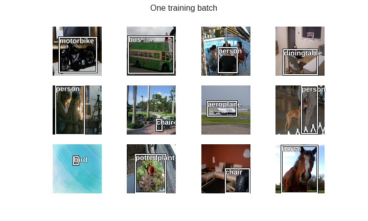
def show_training_batch(batch_num):
trn_iter = iter(md.trn_dl)
for i in range(batch_num):
next(trn_iter)
x,y = next(trn_iter)
fig, axes = plt.subplots(3, 4, figsize=(10, 6))
fig.suptitle('One training batch', fontsize=16)
for i,ax in enumerate(axes.flat):
ima=md.trn_ds.ds.denorm(to_np(x))[i]
b = bb_hw(to_np(y[0][i]))
ax = show_img(ima, ax=ax)
draw_rect(ax, b)
draw_text(ax, b[:2], md2.classes[y[1][i]])
fig_name = f'training-batch-{batch_num}.png'
plt.savefig(fig_name)
print(f'')
plt.close(fig)
# plt.tight_layout()
show_training_batch(2)
Custom head of the convnet
It’s time to think about the output of this model. The easiest approach is to simply concatenate the outputs of the previous two models, ie, 4 activations for a bounding box, and a number of classes activations for classification. We’ll add one more linear layer to the custom head this time, with ReLU, Dropout, and BatchNorm where appropriate.
head_reg4 = nn.Sequential(
    Flatten(),
    nn.ReLU(),
    nn.Dropout(0.5),
    nn.Linear(512*7*7,256),
    nn.ReLU(),
    nn.BatchNorm1d(256),
    nn.Dropout(0.5),
    nn.Linear(256,4+len(cats)),
)
models = ConvnetBuilder(f_model, 0, 0, 0, custom_head=head_reg4)

learn = ConvLearner(md, models)
learn.opt_fn = optim.Adam
Here’s the custom head we added to the backbone.
learn.model[8]
Sequential(
  (0): Flatten(
  )
  (1): ReLU()
  (2): Dropout(p=0.5)
  (3): Linear(in_features=25088, out_features=256, bias=True)
  (4): ReLU()
  (5): BatchNorm1d(256, eps=1e-05, momentum=0.1, affine=True)
  (6): Dropout(p=0.5)
  (7): Linear(in_features=256, out_features=24, bias=True)
)
Loss function and metrics
This custom architecture needs a custom loss function. As per the Dataset created above, the ground truth y is a tuple containing (bounding_box,class) so we can destructure it directly into two variables bb_targ and c_targ. The predictions coming from the network is a tensor of shape (batch_size,4+len(categories)), so we can create two variables bb_inp, c_inp by indexing into this tensor. Once we have these 4 variables, it basically a combination of the two kinds of losses used before:
- L1 loss for bounding box variables
- Cross entropy for classification variables
In order to make it easier for the model to converge, we scale the bounding box predictions to fit in the range of (0,224) (224 being the dimension of the image) by first performing a sigmoid (which scales it to (0,1)), and then multiplying by 224. Also, the cross-entropy loss is multiplied by a factor (20 in this case) to bring the two losses on the same scale.
def detn_loss(input, target):
    bb_targ,c_targ = target
    bb_inp,c_inp = input[:, :4], input[:, 4:]

    bb_inp = F.sigmoid(bb_inp)*224

    return F.l1_loss(bb_inp, bb_targ) + F.cross_entropy(c_inp, c_targ)*20
We can also write custom loss metrics for each task. These will show up during training.
def detn_l1(input, target):
    bb_targ,_ = target
    bb_inp = input[:, :4]
    bb_inp = F.sigmoid(bb_inp)*224
    return F.l1_loss(V(bb_inp),V(bb_targ)).data

def detn_acc(input, target):
    _,c_targ = target
    c_inp = input[:, 4:]
    return accuracy(c_inp, c_targ)
learn.crit = detn_loss
learn.metrics = [detn_acc, detn_l1]
Training
learn.lr_find()
learn.sched.plot()
97%|█████████▋| 31/32 [00:36<00:00, 2.54it/s, loss=601]
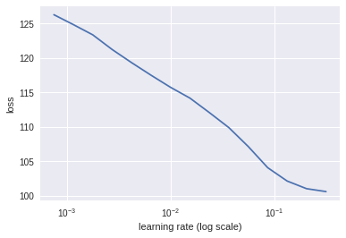
lr=1e-2
learn.fit(lr, 1, cycle_len=3, use_clr=(32,5))
epoch      trn_loss   val_loss   detn_acc   detn_l1
    0      72.976483  44.597288  0.79       31.657924
    1      53.448595  36.711062  0.826      25.718313
    2      44.457675  35.144379  0.84       24.485125
[array([35.14438]), 0.8399999976158142, 24.485124588012695]
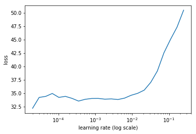
learn.freeze_to(-2)
lrs = np.array([lr/100, lr/10, lr])
learn.lr_find(lrs/1000)
learn.sched.plot(0)
91%|█████████ | 29/32 [00:09<00:01, 2.99it/s, loss=308]
learn.fit(lrs/5, 1, cycle_len=5, use_clr=(32,10))
epoch      trn_loss   val_loss   detn_acc   detn_l1
    0      37.499393  35.342807  0.79       22.659201
    1      32.100903  32.894774  0.828      21.364469
    2      27.395781  31.612098  0.83       20.496989
    3      24.118376  30.928467  0.84       19.8688
    4      21.751545  30.357756  0.836      19.526993
[array([30.35776]), 0.8360000023841858, 19.52699264526367]
learn.unfreeze()
learn.fit(lrs/10, 1, cycle_len=10, use_clr=(32,10))
epoch      trn_loss   val_loss   detn_acc   detn_l1
    0      19.095751  31.384051  0.814      19.595566
    1      18.454536  30.605338  0.822      19.458042
    2      17.760305  30.329738  0.828      19.527608
    3      16.92527   29.743063  0.828      18.627137
    4      16.159306  30.282852  0.832      18.666305
    5      15.2422    30.32975   0.822      18.639726
Getting similar metrics as before for both tasks, ie, around 80% accuracy for classification, and L1 loss of about 18 for localization.
One takeaway here is that the computation performed by the convnet to find “which” is the largest object in the image is shared with that to find “where” is this object. Earlier the largest object classifier and largest object localizer were working in isolation, but here it’s a single network performing both tasks.
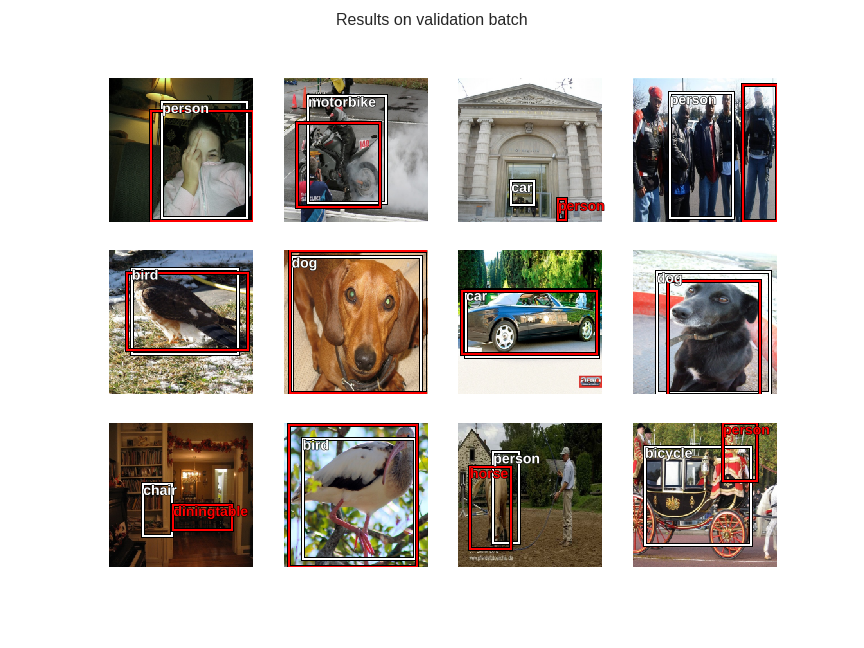
Let’s check out the results on validation set.
from scipy.special import expit
def show_validation_batch(batch_num):
val_iter = iter(md.val_dl)
for i in range(batch_num):
next(val_iter)
x,ground_truth = next(val_iter)
learn.model.eval()
preds = to_np(learn.model(VV(x)))
fig, axes = plt.subplots(3, 4, figsize=(12, 9))
fig.suptitle('Results on validation batch', fontsize=16)
for i,ax in enumerate(axes.flat):
ima=md.val_ds.ds.denorm(to_np(x))[i]
bb = expit(preds[i][:4])*224
predicted_bb = bb_hw(bb)
predicted_class = np.argmax(preds[i][4:])
actual_bb = bb_hw(to_np(ground_truth[0][i]))
actual_class = ground_truth[1][i]
ax = show_img(ima, ax=ax)
# draw prediction
draw_rect(ax, predicted_bb)
draw_text(ax, predicted_bb[:2], md2.classes[predicted_class])
# draw ground truth
draw_rect(ax, actual_bb, color="red")
if not predicted_class == actual_class:
draw_text(ax, actual_bb[:2], md2.classes[actual_class], color="red")
fig_name = f'validation-batch-{batch_num}.png'
plt.savefig(fig_name)
print(f'')
plt.close(fig)
# plt.tight_layout()
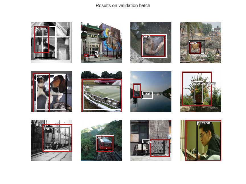
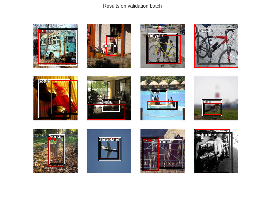
The white bounding boxes and text correspond to predictions, and the red ones correspond to the ground truth. Multiple labels are shown only when the model mis-classifies the largest object.
show_validation_batch(1)
show_validation_batch(2)
show_validation_batch(3)
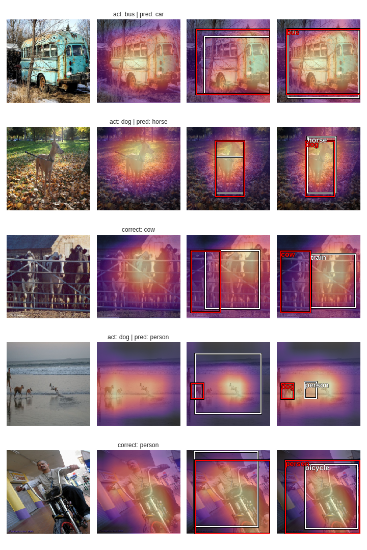
Now that we have models for all three stages, let’s compare heat-maps from forward activations for all of them.
learn_classifier_only = ConvLearner.pretrained(f_model, md2, metrics=[accuracy])
learn_classifier_only.opt_fn = optim.Adam
learn_classifier_only.load('clas_one')
md_localizer = ImageClassifierData.from_csv(PATH, JPEGS, BB_CSV, tfms=tfms,
   bs=bs, continuous=True, val_idxs=val_idxs)
head_reg4 = nn.Sequential(Flatten(), nn.Linear(512*7*7,4))

learn_localizer_only = ConvLearner.pretrained(f_model, md_localizer, custom_head=head_reg4)
learn_localizer_only.opt_fn = optim.Adam
learn_localizer_only.load('reg4')
m_classifier_only = learn_classifier_only.model.eval();
m_localizer_only = learn_localizer_only.model.eval();
m_both = learn.model.eval();
def save_outputs_classifier(self, input, output):
    outputs_classifier.append(output.data)

def save_outputs_localizer(self, input, output):
    outputs_localizer.append(output.data)

def save_outputs_both(self, input, output):
    outputs_both.append(output.data)
last_conv_hook_handle_cl = m_classifier_only[7].register_forward_hook(save_outputs_classifier)
last_conv_hook_handle_lo = m_localizer_only[7].register_forward_hook(save_outputs_localizer)
last_conv_hook_handle_both = m_both[7].register_forward_hook(save_outputs_both)
def results_from_all_three_stages(batch_num, num_rows, miss_classified_only=True):
val_iter = iter(md.val_dl)
for i in range(batch_num):
next(val_iter)
x,ground_truth = next(val_iter)
learn.model.eval()
learn_classifier_only.model.eval()
learn_localizer_only.model.eval()
probs_stage_1 = F.softmax(predict_batch(learn_classifier_only.model, x), -1)
preds_stage_1 = to_np(probs_stage_1)
preds_stage_1 = np.argmax(preds_stage_1, -1)
preds_stage_2 = to_np(learn_localizer_only.model(VV(x)))
preds_stage_3 = to_np(learn.model(VV(x)))
x = to_np(x)
acts1 = outputs_classifier[0].cpu()
avg_acts1 = acts1.mean(1)
acts2 = outputs_localizer[0].cpu()
avg_acts2 = acts2.mean(1)
acts3 = outputs_both[0].cpu()
avg_acts3 = acts3.mean(1)
fig, axes = plt.subplots(num_rows, 4, figsize=(10, num_rows*3))
# fig.suptitle('Results from all three stages', fontsize=16)
i = 0
for j in range(x.shape[0]):
if i==num_rows:
break
ima=md.val_ds.ds.denorm(to_np(x))[j]
bb = expit(preds_stage_3[j][:4])*224
predicted_bb = bb_hw(bb)
predicted_class = np.argmax(preds_stage_3[j][4:])
actual_bb = bb_hw(to_np(ground_truth[0][j]))
actual_class = ground_truth[1][j]
if not predicted_class == actual_class or not miss_classified_only: # only plotting images where classifier is incorrect
# 1st column
axes[i,0] = show_img(ima, ax=axes[i,0])
# 2nd column
axes[i,1] = show_img(ima, ax=axes[i,1])
b = md2.classes[preds_stage_1[j]]
axes[i,1].imshow(avg_acts1[j], alpha=0.6, extent=(0,224,224,0),
interpolation='bilinear', cmap='magma');
if not md2.classes[actual_class]==b:
axes[i,1].set_title(f'act: {md2.classes[actual_class]} | pred: {b}')
else:
axes[i,1].set_title(f'correct: {b}')
# 3rd column
b_stage_2 = bb_hw(preds_stage_2[i])
axes[i,2] = show_img(ima, ax=axes[i,2])
draw_rect(axes[i,2], b_stage_2)
draw_rect(axes[i,2], actual_bb, color="red")
axes[i,2].imshow(avg_acts2[j], alpha=0.6, extent=(0,224,224,0),
interpolation='bilinear', cmap='magma');
# 4th column
axes[i,3] = show_img(ima, ax=axes[i,3])
draw_rect(axes[i,3], predicted_bb)
draw_text(axes[i,3], predicted_bb[:2], md2.classes[predicted_class])
draw_rect(axes[i,3], actual_bb, color="red")
if not predicted_class == actual_class:
draw_text(axes[i,3], actual_bb[:2], md2.classes[actual_class], color="red")
axes[i,3].imshow(avg_acts3[j], alpha=0.6, extent=(0,224,224,0),
interpolation='bilinear', cmap='magma');
i+=1
plt.tight_layout()
fig_name = f'3-stages-heatmaps-batch-{batch_num}.png'
plt.savefig(fig_name)
plt.close(fig)
print(f'')
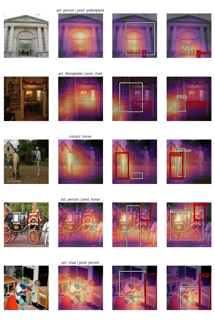
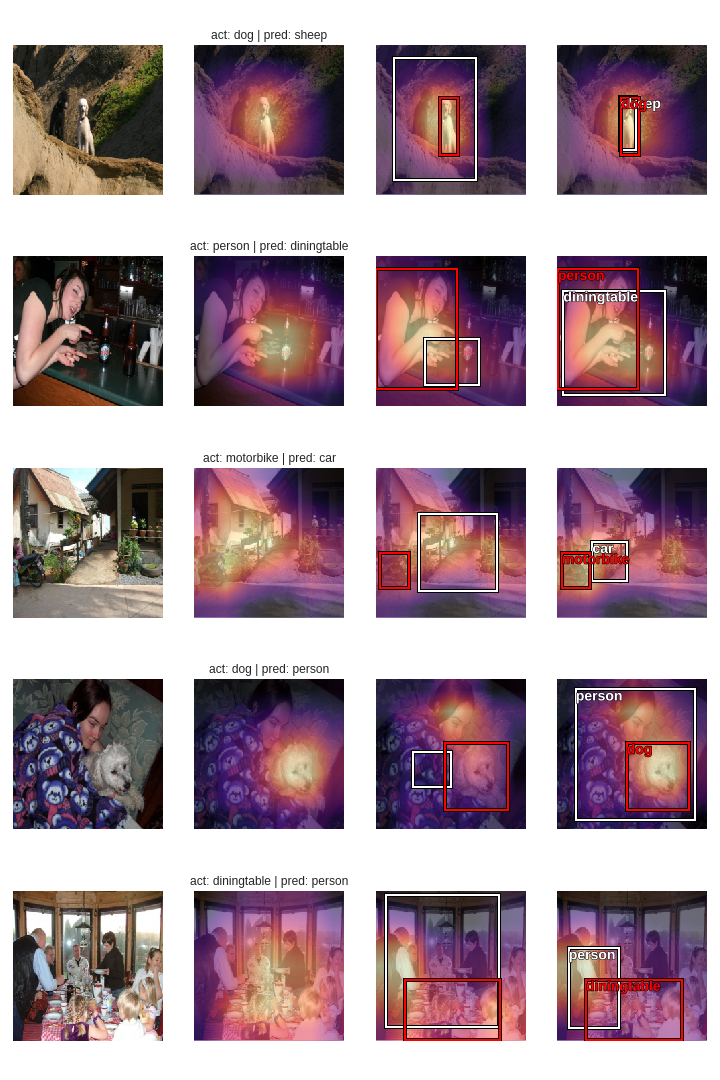
The plots follow the following convention:
- Column 1: original image
- Column 2: Stage 1- classifier only
- Column 3: Stage 2- localizer only
- Column 4: Stage 3 - both classification and localization
White boxes and labels are predictions, while the same in red is ground truth.
outputs_classifier = []
outputs_localizer = []
outputs_both = []
results_from_all_three_stages(1,5)
outputs_classifier = []
outputs_localizer = []
outputs_both = []
results_from_all_three_stages(2,5)
outputs_classifier = []
outputs_localizer = []
outputs_both = []
results_from_all_three_stages(3,5)
Since posting a whole bunch of images on the blog isn’t feasible, I’ve run these experiments on a much bigger set here and here. These notebooks are quite big in size so I recommend viewing them on nbviewer.
It seems that combining both tasks in a single network has mildly modified the behaviour of both tasks individually. Also, the heat-maps for stage 2 and stage 3 are almost similar, but the bounding boxes in stage 3 seem to be quite different than those in stage 2. The model is obviously performing poorly on images containing more than one clearly visible objects.
This concludes single object detection. I’ll resume this exploration with multiple objects detection in upcoming posts.