This post is fourth in a series on object detection. The other posts can be found here, here, and here.
The last post covered use of anchor boxes for detecting multiple objects in an image. I ended that one with a model that was doing fine with detecting the presence of various objects, but the predicted bounding boxes were not able to properly localize objects with non-squared shapes. This post will detail techniques for further improving that baseline model.
The approach used below is based on learnings from fastai’s Deep Learning MOOC (Part 2).
pip install -q fastai==0.7.0 torchtext==0.2.3
!wget -qq http://pjreddie.com/media/files/VOCtrainval_06-Nov-2007.tar
!tar -xf VOCtrainval_06-Nov-2007.tar
!wget -qq https://storage.googleapis.com/coco-dataset/external/PASCAL_VOC.zip
!unzip -q PASCAL_VOC.zip
!mkdir -p data/pascal
!mv PASCAL_VOC/* data/pascal
!mv VOCdevkit data/pascal
%matplotlib inline
%reload_ext autoreload
%autoreload 2
from fastai.conv_learner import *
from fastai.dataset import *

import json, pdb
from PIL import ImageDraw, ImageFont
from matplotlib import patches, patheffects
PATH = Path('data/pascal')
trn_j = json.load((PATH / 'pascal_train2007.json').open())
IMAGES,ANNOTATIONS,CATEGORIES = ['images', 'annotations', 'categories']
FILE_NAME,ID,IMG_ID,CAT_ID,BBOX = 'file_name','id','image_id','category_id','bbox'

cats = dict((o[ID], o['name']) for o in trn_j[CATEGORIES])
trn_fns = dict((o[ID], o[FILE_NAME]) for o in trn_j[IMAGES])
trn_ids = [o[ID] for o in trn_j[IMAGES]]

JPEGS = 'VOCdevkit/VOC2007/JPEGImages'
IMG_PATH = PATH/JPEGS
Setup
Importing all the necessary functions from last time so as to save some space.
from helper_functions import *
!mkdir -p {PATH}/tmp

trn_anno = get_trn_anno()
CLAS_CSV = PATH/'tmp/clas.csv'
MBB_CSV = PATH/'tmp/mbb.csv'

f_model=resnet34
sz=224
bs=64

mc = [[cats[p[1]] for p in trn_anno[o]] for o in trn_ids]
id2cat = list(cats.values())
cat2id = {v:k for k,v in enumerate(id2cat)}
mcs = np.array([np.array([cat2id[p] for p in o]) for o in mc])
val_idxs = get_cv_idxs(len(trn_fns))
((val_mcs,trn_mcs),) = split_by_idx(val_idxs, mcs)

mbb = [np.concatenate([p[0] for p in trn_anno[o]]) for o in trn_ids]
mbbs = [' '.join(str(p) for p in o) for o in mbb]

df = pd.DataFrame({'fn': [trn_fns[o] for o in trn_ids], 'bbox': mbbs}, columns=['fn','bbox'])
df.to_csv(MBB_CSV, index=False)
aug_tfms = [RandomRotate(3, p=0.5, tfm_y=TfmType.COORD),
            RandomLighting(0.05, 0.05, tfm_y=TfmType.COORD),
            RandomFlip(tfm_y=TfmType.COORD)]
tfms = tfms_from_model(f_model, sz, crop_type=CropType.NO, tfm_y=TfmType.COORD, aug_tfms=aug_tfms)
md = ImageClassifierData.from_csv(PATH, JPEGS, MBB_CSV, tfms=tfms, bs=bs,val_idxs=val_idxs, continuous=True, num_workers=4)

trn_ds2 = ConcatLblDataset(md.trn_ds, trn_mcs)
val_ds2 = ConcatLblDataset(md.val_ds, val_mcs)
md.trn_dl.dataset = trn_ds2
md.val_dl.dataset = val_ds2
import matplotlib.cm as cmx
import matplotlib.colors as mcolors
from cycler import cycler

num_colr = 12
cmap = get_cmap(num_colr)
colr_list = [cmap(float(x)) for x in range(num_colr)]
loss_f = BCE_Loss(len(id2cat))
Current status of model
Till now we’ve only used the final convolutional feature maps of grid size (4 x 4) for 16 anchor boxes, which are of a fixed size and a fixed aspect ratio. Since the activations coming from the model can only modify the shape of these anchor boxes by 50%, the predicted bounding boxes can only do a good job on objects which are similar in size to these anchor boxes. Hence, as seen in the validation results last time, the model is not able to properly localize an object which is larger in size than the maximum possible bounding box.
One way to solve this problem would be to start with anchor boxes of varied shapes and sizes to begin with. We can also have these anchors lie on grids corresponding to different scales. Last time we had 16 anchors on a 4 x 4 grid. We can allow prediction of detections at multiple scales by adding more convolutional layers in the custom head and using their activations for predictions. So this time we’ll use activations from the convolutional feature maps of grid sizes 4 x 4, 2 x 2, and 1 x 1.
Let’s create more anchor boxes.
anc_grids = [4,2,1]
anc_zooms = [0.7, 1., 1.3]
anc_ratios = [(1.,1.), (1.,0.5), (0.5,1.)]
anchor_scales = [(anz*i,anz*j) for anz in anc_zooms for (i,j) in anc_ratios]
k = len(anchor_scales)
anc_offsets = [1/(o*2) for o in anc_grids]
anc_x = np.concatenate([np.repeat(np.linspace(ao, 1-ao, ag), ag)
                        for ao,ag in zip(anc_offsets,anc_grids)])
anc_y = np.concatenate([np.tile(np.linspace(ao, 1-ao, ag), ag)
                        for ao,ag in zip(anc_offsets,anc_grids)])
anc_ctrs = np.repeat(np.stack([anc_x,anc_y], axis=1), k, axis=0)
anc_sizes  =   np.concatenate([np.array([[o/ag,p/ag] for i in range(ag*ag) for o,p in anchor_scales])
               for ag in anc_grids])
grid_sizes = V(np.concatenate([np.array([ 1/ag       for i in range(ag*ag) for o,p in anchor_scales])
               for ag in anc_grids]), requires_grad=False).unsqueeze(1)
anchors = V(np.concatenate([anc_ctrs, anc_sizes], axis=1), requires_grad=False).float()
anchor_cnr = hw2corners(anchors[:,:2], anchors[:,2:])
print(k)
9
We have 9 variants of an anchor box at a given grid cell location.
16*k + 4*k +1*k
189
anchors.shape
torch.Size([189, 4])
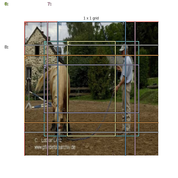
We have a total of 189 anchor boxes this time. Let’s plot them on an image to see how they look.
itr = iter(md.val_dl)
next(itr)
x,y = next(itr)
ima=md.val_ds.ds.denorm(to_np(x))[10]
As mentioned above the last 9 anchor boxes correspond to a (1 x 1) grid.
fig, ax = plt.subplots(figsize=(8,8))
torch_gt(ax, ima, anchor_cnr[-1*k:], None);
ax.set_title('1 x 1 grid');
fig_name = f'plots-1.png'
plt.savefig(fig_name)
print(f'')
plt.close(fig)
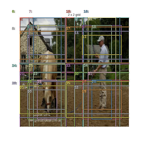
Looks good. Let’s plot the 36 anchor boxes corresponding to a (2 x 2) grid.
fig, ax = plt.subplots(figsize=(8,8))
torch_gt(ax, ima, anchor_cnr[16*k:16*k+4*k], None);
ax.set_title('2 x 2 grid');
fig_name = f'plots-2.png'
plt.savefig(fig_name)
print(f'')
plt.close(fig)
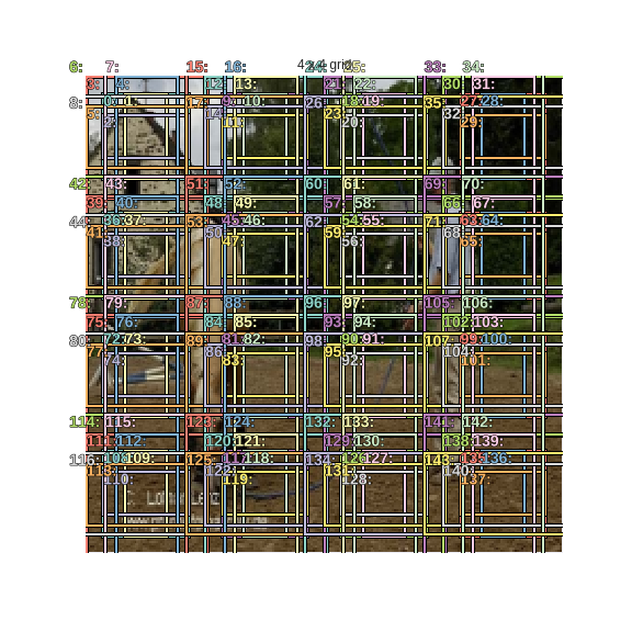
Finally, the 144 anchor boxes corresponding to (4 x 4) grid.
fig, ax = plt.subplots(figsize=(8,8))
torch_gt(ax, ima, anchor_cnr[:16*k], None);
ax.set_title('4 x 4 grid');
fig_name = f'plots-3.png'
plt.savefig(fig_name)
print(f'')
plt.close(fig)
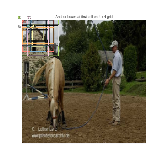
That’s a lot of anchor boxes. Let’s just plot the 9 corresponding to the first cell.
fig, ax = plt.subplots(figsize=(8,8))
torch_gt(ax, ima, anchor_cnr[:9], None);
ax.set_title('Anchor boxes at first cell on 4 x 4 grid');
fig_name = f'plots-4.png'
plt.savefig(fig_name)
print(f'')
plt.close(fig)
Finally, let’s plot all 9 variations on different grid locations so as to see the difference clearly. The corresponding anchor scaling is also plotted.
i = 0
l = []
for j in range(9):
    l.append(j*9+j)
print(l)
[0, 10, 20, 30, 40, 50, 60, 70, 80]
fig, ax = plt.subplots(figsize=(8,8))
torch_gt(ax, ima, anchor_cnr[l], None, forced_text=anchor_scales);
fig_name = f'plots-5.png'
plt.savefig(fig_name)
print(f'')
plt.close(fig)

By using all of these 189 anchor boxes we now have a much better chance of detecting objects of varying shapes and sizes. Time to modify the custom head.
Custom head
As mentioned above, we need to add 2 more convolutional layers with stride 2 and use the activations coming from all 4 layers for predictions. Copying the custom convolutional modules from last time.
class StdConv(nn.Module):
    def __init__(self, nin, nout, stride=2, drop=0.1):
        super().__init__()
        self.conv = nn.Conv2d(nin, nout, 3, stride=stride, padding=1)
        self.bn = nn.BatchNorm2d(nout)
        self.drop = nn.Dropout(drop)

    def forward(self, x): return self.drop(self.bn(F.relu(self.conv(x))))

def flatten_conv(x,k):
    bs,nf,gx,gy = x.size()
    x = x.permute(0,2,3,1).contiguous()
    return x.view(bs,-1,nf//k)

class OutConv(nn.Module):
    def __init__(self, k, nin, bias):
        super().__init__()
        self.k = k
        self.oconv1 = nn.Conv2d(nin, (len(id2cat)+1)*k, 3, padding=1)
        self.oconv2 = nn.Conv2d(nin, 4*k, 3, padding=1)
        self.oconv1.bias.data.zero_().add_(bias)

    def forward(self, x):
        return [flatten_conv(self.oconv1(x), self.k),
                flatten_conv(self.oconv2(x), self.k)]
The ResNet backbone results in a tensor of shape (64,512,7,7). Let’s put it through a Conv2d with stride 1 and 256 output planes.
cnv_512 = StdConv(512,256,stride=1)
cnv_256 = StdConv(256,256)
output_from_backbone = Variable(torch.randn(64,512,7,7))
out_cnv = OutConv(k, 256, -4.)
conv_out_1 = cnv_256(cnv_512(output_from_backbone))
conv_out_1.shape
torch.Size([64, 256, 4, 4])
out1 = out_cnv(conv_out_1)
out1[0].shape,out1[1].shape
(torch.Size([64, 144, 21]), torch.Size([64, 144, 4]))
The above are the first set of activations that we’ll use for predictions and these correspond to a 441 anchor boxes on a grid size of (7 x 7).
Next, let’s have a convolutional layer with stride 2 that brings the feature map dimensions down to 4 x 4.
conv_out_2 = cnv_256(conv_out_1)
conv_out_2.shape
torch.Size([64, 256, 2, 2])
out2 = out_cnv(conv_out_2)
out2[0].shape,out2[1].shape
(torch.Size([64, 36, 21]), torch.Size([64, 36, 4]))
The above are the second set of activations that we’ll use for predictions and these correspond to a 144 anchor boxes on a grid size of (4 x 4).
Next, let’s have the final convolutional layer with stride 2 which result in feature maps of grid size (1 x 1).
conv_out_3 = cnv_256(conv_out_2)
conv_out_3.shape
torch.Size([64, 256, 1, 1])
out3 = out_cnv(conv_out_3)
out3[0].shape,out3[1].shape
(torch.Size([64, 9, 21]), torch.Size([64, 9, 4]))
The above are the third set of activations that we’ll use for predictions and these correspond to 9 anchor boxes on a grid size of (1 x 1).
So we’ve changed the architecture from last time by adding 2 more convolutional layers. This model will concatenate these tensors and output a list of two tensors containing 189 sets of activations for both classification and localization as compared to 16 earlier.
torch.cat([out1[0],out2[0],out3[0]], dim=1).shape
torch.Size([64, 189, 21])
torch.cat([out1[1],out2[1],out3[1]], dim=1).shape
torch.Size([64, 189, 4])
Let’s put all of this in a single module.
drop=0.4

class SSD_MultiHead(nn.Module):
    def __init__(self, k, bias):
        super().__init__()
        self.drop = nn.Dropout(drop)
        self.sconv0 = StdConv(512,256, stride=1, drop=drop)
        self.sconv1 = StdConv(256,256, drop=drop)
        self.sconv2 = StdConv(256,256, drop=drop)
        self.sconv3 = StdConv(256,256, drop=drop)
        self.out0 = OutConv(k, 256, bias)
        self.out1 = OutConv(k, 256, bias)
        self.out2 = OutConv(k, 256, bias)
        self.out3 = OutConv(k, 256, bias)

    def forward(self, x):
        x = self.drop(F.relu(x))
        x = self.sconv0(x)
        x = self.sconv1(x)
        o1c,o1l = self.out1(x)
        x = self.sconv2(x)
        o2c,o2l = self.out2(x)
        x = self.sconv3(x)
        o3c,o3l = self.out3(x)
        return [torch.cat([o1c,o2c,o3c], dim=1),
                torch.cat([o1l,o2l,o3l], dim=1)]
That’s it for the architecture. The 189 anchor boxes are arranged in the order corresponding to the activations coming from the network, which means that the loss function ssd_loss from last time can be used without any modifications since the activations and anchor boxes are mapped one-to-one.
Training
head_reg4 = SSD_MultiHead(k, -4.)
models = ConvnetBuilder(f_model, 0, 0, 0, custom_head=head_reg4)
learn = ConvLearner(md, models)
learn.opt_fn = optim.Adam
learn.crit = ssd_loss
lr = 1e-2
lrs = np.array([lr/100,lr/10,lr])
learn.lr_find(lrs/1000,1.)
learn.sched.plot(n_skip_end=2)
learn.fit(lrs, 1, cycle_len=4, use_clr=(20,8))
epoch      trn_loss   val_loss
    0      22.98593   23.285165
    1      19.25035   15.106181
    2      16.641781  13.666947
    3      14.801657  13.034863
[array([13.03486])]
learn.freeze_to(-2)
learn.fit(lrs/2, 1, cycle_len=4, use_clr=(20,8))
epoch      trn_loss   val_loss
    0      14.148568  17.447378
    1      13.448161  12.855588
    2      12.329596  11.981028
    3      11.378326  11.402132
[array([11.40213])]
Let’s take a look at the results.
def show_validation_batch(batch_num, show_bg=False, thresh=0.01):
val_iter = iter(md.val_dl)
for i in range(batch_num):
next(val_iter)
x,y = next(val_iter)
fig, axes = plt.subplots(4, 3, figsize=(12, 16))
x,y = V(x),V(y)
learn.model.eval()
batch = learn.model(x)
b_clas,b_bb = batch
for idx,ax in enumerate(axes.flat):
b_clasi = b_clas[idx]
b_bboxi = b_bb[idx]
ima=md.val_ds.ds.denorm(to_np(x))[idx]
bbox,clas = get_y(y[0][idx], y[1][idx])
a_ic = actn_to_bb(b_bb[idx], anchors)
overlaps = jaccard(bbox.data, anchor_cnr.data)
gt_overlap,gt_idx = map_to_ground_truth(overlaps)
gt_clas = clas[gt_idx]
pos = gt_overlap > thresh
pos_idx = torch.nonzero(pos)[:,0]
gt_clas[1-pos] = len(id2cat)
not_bg = (b_clasi.max(1)[1]!=len(id2cat)).nonzero().view(-1)
if show_bg:
torch_gt(ax, ima, a_ic, b_clasi.max(1)[1], b_clasi.max(1)[0].sigmoid(), thresh=thresh);
else:
torch_gt(ax, ima, a_ic[not_bg], b_clasi.max(1)[1][not_bg], b_clasi.max(1)[0][not_bg].sigmoid(), thresh=thresh);
plt.tight_layout()
fig_name = f'plots-6-batch-{batch_num}.png'
plt.savefig(fig_name)
print(f'')
plt.close(fig)
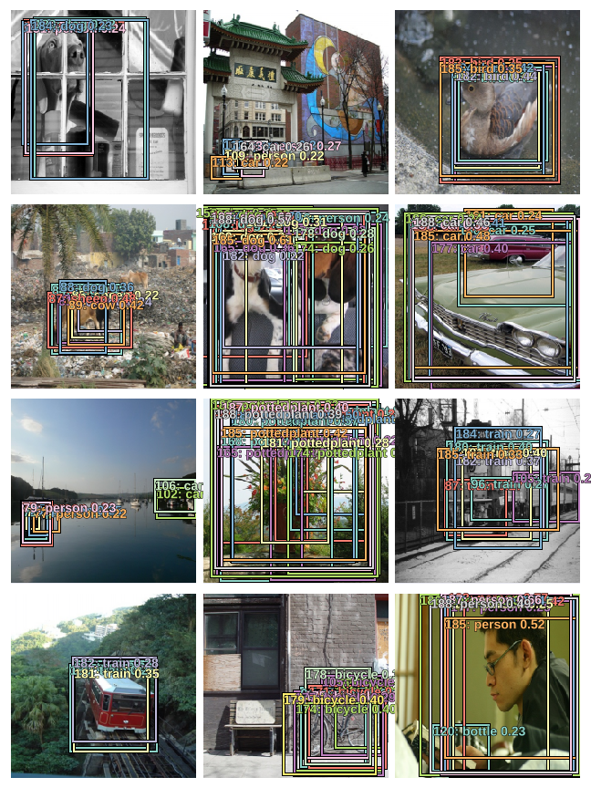
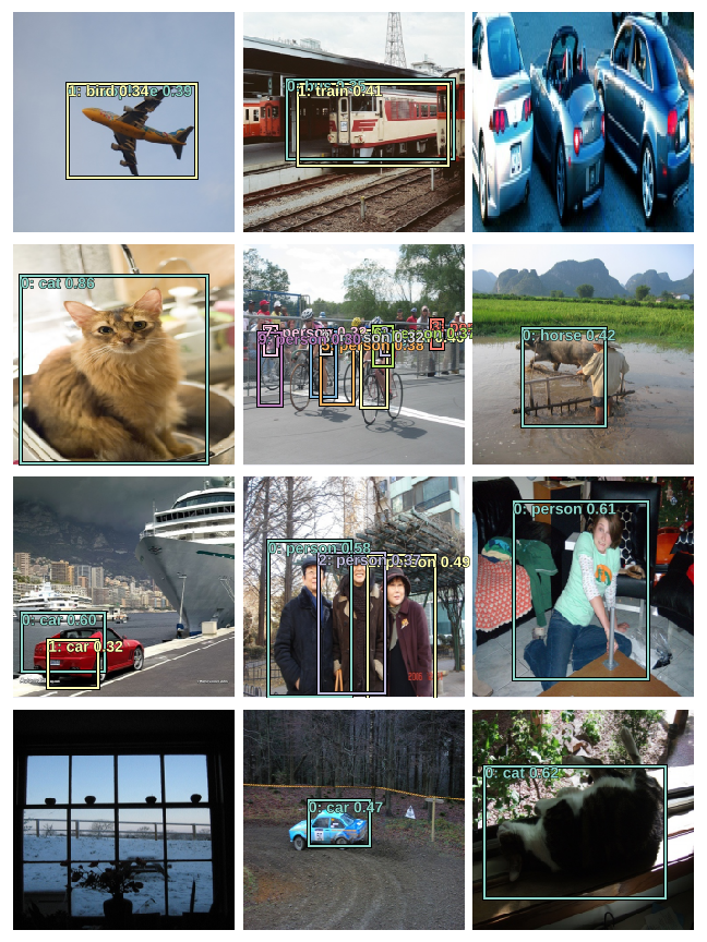
show_validation_batch(1, thresh=0.2)
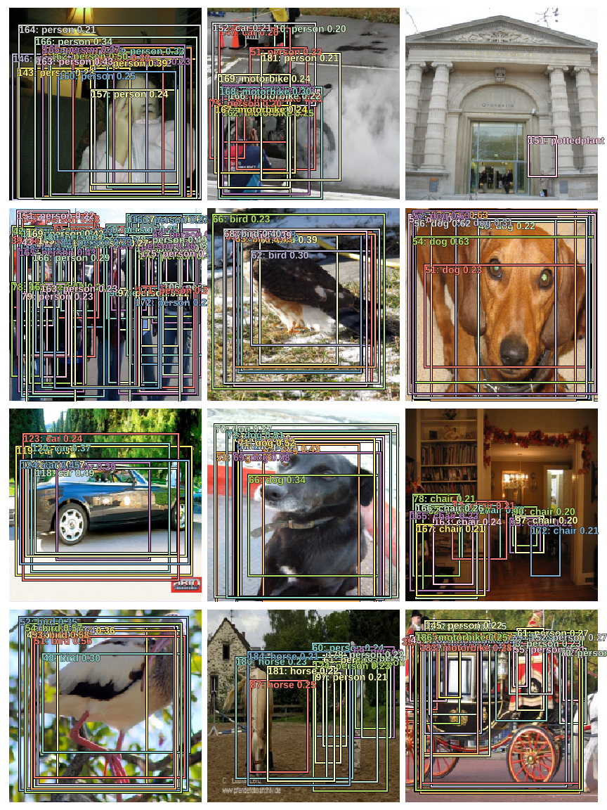
show_validation_batch(2, thresh=0.2)
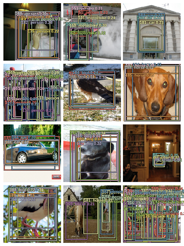
Let’s compare the above with the results from last time.
Results from last time:
As evident from the images above, the model is doing better than last time, especially on large objects. This is the result of using anchor boxes of different shapes at multiple scales.
Using Focal loss
The loss criterion ssd_loss uses BCE_Loss as the classification loss criteria as defined above. Let’s use focal loss instead of the standard cross-entropy loss to get better results. We can do that by simple overriding the get_weight method defined in the BCE_Loss class.
class FocalLoss(BCE_Loss):
    def get_weight(self,x,t):
        alpha,gamma = 0.25,2
        p = x.sigmoid()
        pt = p*t + (1-p)*(1-t)
        w = alpha*t + (1-alpha)*(1-t)
        return w * (1-pt).pow(gamma)
loss_f = FocalLoss(len(id2cat))
learn.lr_find(lrs/1000,1.)
learn.sched.plot(n_skip_end=1)
learn.fit(lrs, 1, cycle_len=10, use_clr=(20,10))
epoch      trn_loss   val_loss
    0      12.296044  17.881611
    1      14.069504  16.269705
    2      13.887531  16.88969
    3      13.093471  12.81302
    4      12.106579  12.44246
    5      11.986497  15.610915
    6      11.87363   12.373115
    7      11.143738  11.851826
    8      10.382161  11.40408
    9      9.791606   11.260116
[array([11.26012])]
learn.save('multi_anchor_189_stage_1')
learn.freeze_to(-2)
learn.fit(lrs/4, 1, cycle_len=10, use_clr=(20,10))
epoch      trn_loss   val_loss
    0      9.087099   11.899447
    1      8.991511   11.448938
    2      8.805311   11.275349
    3      8.51155    11.397906
    4      8.232354   11.15149
    5      7.943597   11.154927
    6      7.654771   10.989628
    7      7.411221   10.947957
    8      7.210082   10.893854
    9      7.038593   10.870361
[array([10.87036])]
learn.save('multi_anchor_189_final')
def plot_results(batch_num, thresh):
val_iter = iter(md.val_dl)
for i in range(batch_num):
next(val_iter)
x,y = next(val_iter)
y = V(y)
batch = learn.model(V(x))
b_clas,b_bb = batch
x = to_np(x)
fig, axes = plt.subplots(4, 3, figsize=(9, 12))
for idx,ax in enumerate(axes.flat):
ima=md.val_ds.ds.denorm(x)[idx]
bbox,clas = get_y(y[0][idx], y[1][idx])
a_ic = actn_to_bb(b_bb[idx], anchors)
clas_pr, clas_ids = b_clas[idx].max(1)
clas_pr = clas_pr.sigmoid()
# print(clas_pr.max().data[0]*thresh)
# torch_gt(ax, ima, a_ic, clas_ids, clas_pr, clas_pr.max().data[0]*thresh)
torch_gt(ax, ima, a_ic, clas_ids, clas_pr, thresh)
plt.tight_layout()
fig_name = f'plots-7-batch-{batch_num}.png'
plt.savefig(fig_name)
print(f'')
plt.close(fig)
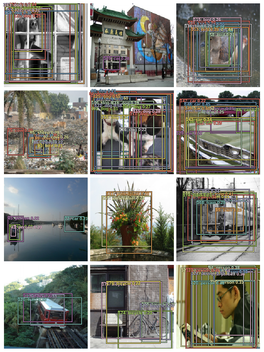
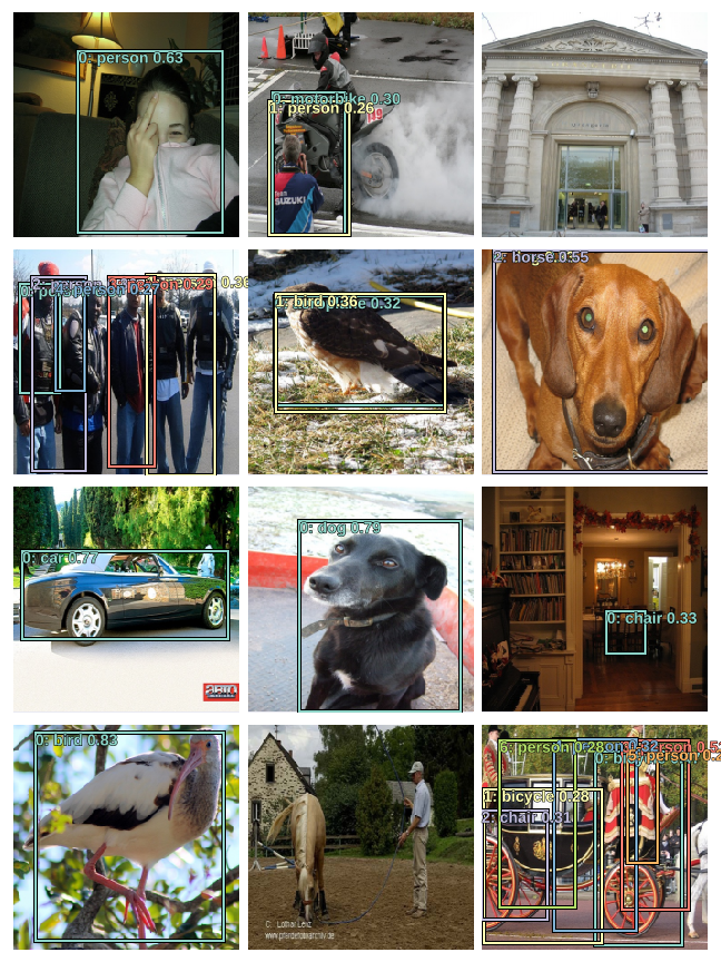
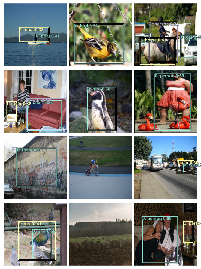
plot_results(1, 0.2)
plot_results(2, 0.2)
Non-Max Suppression
As seen in the results above the model is predicting multiple bounding boxes per object with varying confidences. We need have a mechanism to filter down to the most appropriate bounding box for a given object. This is done by Non-Max Suppression.
First, we filter out most boxes by using a confidence threshold. For the remaining boxes we do this:
- Pick a pair of boxes. If they have a jaccard overlap of more than a threshold and they’re predicting the same class, we’ll assume they’re predicting the same object, and discard the box with lower confidence.
- We do this till we have boxes where no two overlap more than the jaccard threshold.
def nms(boxes, scores, overlap=0.5, top_k=100):
    keep = scores.new(scores.size(0)).zero_().long()
    if boxes.numel() == 0: return keep
    x1 = boxes[:, 0]
    y1 = boxes[:, 1]
    x2 = boxes[:, 2]
    y2 = boxes[:, 3]
    area = torch.mul(x2 - x1, y2 - y1)
    v, idx = scores.sort(0)  # sort in ascending order
    idx = idx[-top_k:]  # indices of the top-k largest vals
    xx1 = boxes.new()
    yy1 = boxes.new()
    xx2 = boxes.new()
    yy2 = boxes.new()
    w = boxes.new()
    h = boxes.new()

    count = 0
    while idx.numel() > 0:
        i = idx[-1]  # index of current largest val
        keep[count] = i
        count += 1
        if idx.size(0) == 1: break
        idx = idx[:-1]  # remove kept element from view
        # load bboxes of next highest vals
        torch.index_select(x1, 0, idx, out=xx1)
        torch.index_select(y1, 0, idx, out=yy1)
        torch.index_select(x2, 0, idx, out=xx2)
        torch.index_select(y2, 0, idx, out=yy2)
        # store element-wise max with next highest score
        xx1 = torch.clamp(xx1, min=x1[i])
        yy1 = torch.clamp(yy1, min=y1[i])
        xx2 = torch.clamp(xx2, max=x2[i])
        yy2 = torch.clamp(yy2, max=y2[i])
        w.resize_as_(xx2)
        h.resize_as_(yy2)
        w = xx2 - xx1
        h = yy2 - yy1
        # check sizes of xx1 and xx2.. after each iteration
        w = torch.clamp(w, min=0.0)
        h = torch.clamp(h, min=0.0)
        inter = w*h
        # IoU = i / (area(a) + area(b) - i)
        rem_areas = torch.index_select(area, 0, idx)  # load remaining areas)
        union = (rem_areas - inter) + area[i]
        IoU = inter/union  # store result in iou
        # keep only elements with an IoU <= overlap
        idx = idx[IoU.le(overlap)]
    return keep, count
def show_batch_with_nms(batch_num, conf_threshold=0.2, jaccard_threshold=0.3):
val_iter = iter(md.val_dl)
for i in range(batch_num):
next(val_iter)
x,y = next(val_iter)
y = V(y)
batch = learn.model(V(x))
b_clas,b_bb = batch
x = to_np(x)
fig, axes = plt.subplots(4, 3, figsize=(9, 12))
for idx,ax in enumerate(axes.flat):
ima=md.val_ds.ds.denorm(x)[idx]
bbox,clas = get_y(y[0][idx], y[1][idx])
a_ic = actn_to_bb(b_bb[idx], anchors)
clas_pr, clas_ids = b_clas[idx].max(1)
clas_pr = clas_pr.sigmoid()
conf_scores = b_clas[idx].sigmoid().t().data
out1,out2,cc = [],[],[]
for cl in range(0, len(conf_scores)-1):
c_mask = conf_scores[cl] > conf_threshold
if c_mask.sum() == 0: continue
scores = conf_scores[cl][c_mask]
l_mask = c_mask.unsqueeze(1).expand_as(a_ic)
boxes = a_ic[l_mask].view(-1, 4)
ids, count = nms(boxes.data, scores, jaccard_threshold, 50)
ids = ids[:count]
out1.append(scores[ids])
out2.append(boxes.data[ids])
cc.append([cl]*count)
if not cc:
# print(f"{idx}: empty array")
ax.imshow(ima)
ax.get_xaxis().set_visible(False)
ax.get_yaxis().set_visible(False)
else:
cc = T(np.concatenate(cc))
out1 = torch.cat(out1)
out2 = torch.cat(out2)
torch_gt(ax, ima, out2, cc, out1, 0.1)
plt.tight_layout()
fig_name = f'plots-8-batch-{batch_num}.png'
plt.savefig(fig_name)
print(f'')
plt.close(fig)
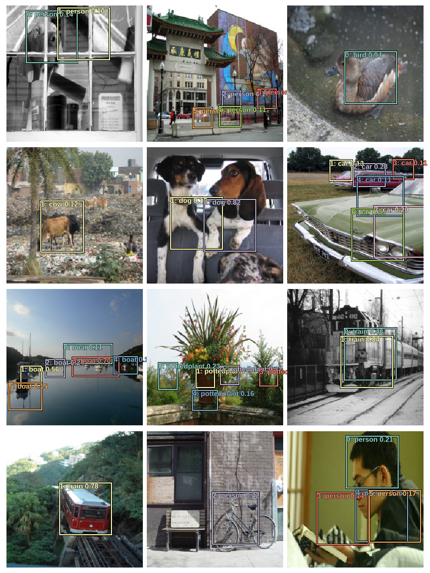
show_batch_with_nms(batch_num=1, conf_threshold=0.25, jaccard_threshold=0.35)
show_batch_with_nms(batch_num=2, conf_threshold=0.25, jaccard_threshold=0.35)
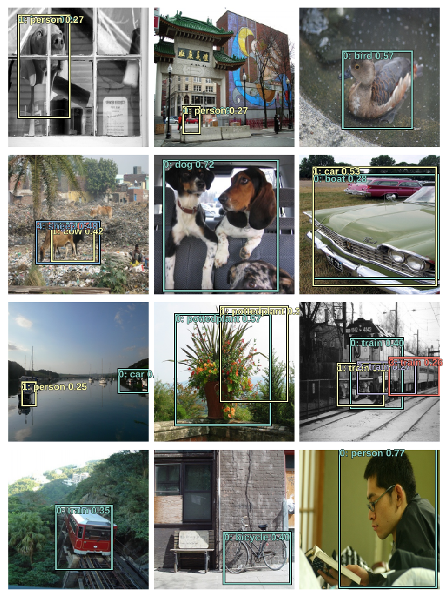
show_batch_with_nms(batch_num=3, conf_threshold=0.25, jaccard_threshold=0.35)
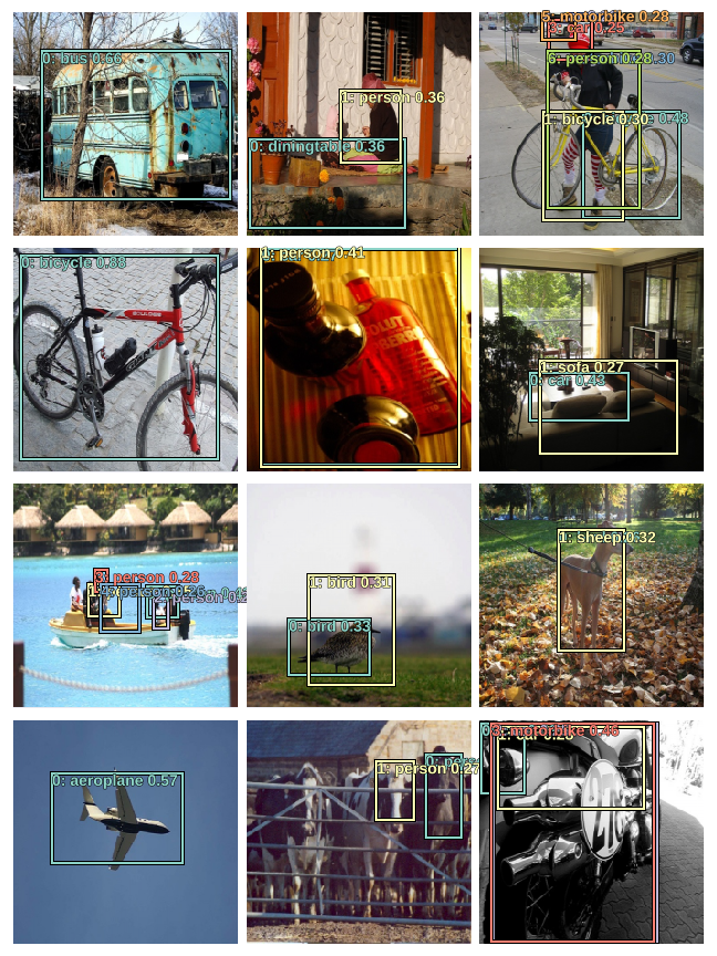
show_batch_with_nms(batch_num=4, conf_threshold=0.25, jaccard_threshold=0.35)

show_batch_with_nms(batch_num=5, conf_threshold=0.3, jaccard_threshold=0.4)
show_batch_with_nms(batch_num=6, conf_threshold=0.3, jaccard_threshold=0.4)
This concludes my initial exploration into the workings of object detection using deep neural networks. It took me a couple of weeks to fully grasp the concepts, and the whole exercise definitely improved my understanding of convnets.