I’m currently learning about Convolutional Neural Nets from deeplearning.ai, and boy are they really powerful. Some of them even have cool names like Inception Network and make use of algorithms like You Only Look Once (YOLO). That is hilarious and awesome.
This notebook/post is an exercise in trying to visualize the outputs of the various layers in a CNN. Let’s get to it.
Setup
import numpy as np
import pandas as pd

from math import ceil
import matplotlib.pyplot as plt
import matplotlib.image as mpimg
from sklearn.model_selection import train_test_split

from keras import layers
from keras.layers import Input, Dense, Activation, ZeroPadding2D, Flatten, Conv2D
from keras.layers import AveragePooling2D, MaxPooling2D
from keras.models import Model
from keras.datasets import fashion_mnist
from keras.optimizers import Adam
from keras.models import load_model
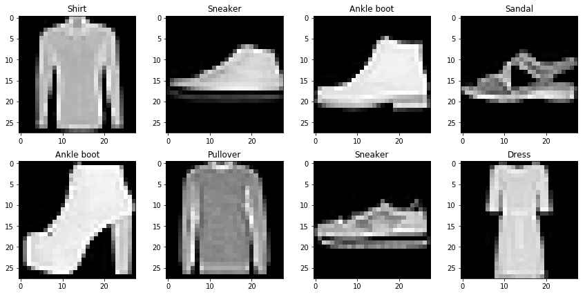
To begin with, I’ll use the Fashion-MNIST dataset.
(x_train_orig, y_train_orig), (x_test_orig, y_test_orig) = fashion_mnist.load_data()
x_train = x_train_orig.reshape(-1, 28, 28, 1)
y_train = np.eye(10)[y_train_orig]
x_test = x_test_orig.reshape(-1, 28, 28, 1)
y_test = np.eye(10)[y_test_orig]
The dataset contains 70,000 grayscale images of shape 28x28.
print(x_train.shape, y_train.shape, x_test.shape, y_test.shape)
(60000, 28, 28, 1) (60000, 10) (10000, 28, 28, 1) (10000, 10)
Each image in this dataset belongs to one of the following classes.
labels = {
        0:"T-shirt/top",
        1:"Trouser",
        2:"Pullover",
        3:"Dress",
        4:"Coat",
        5:"Sandal",
        6:"Shirt",
        7:"Sneaker",
        8:"Bag",
        9:"Ankle boot"
}
Let’s take a look at the images.
fig, axarr = plt.subplots(2, 4)
fig.set_size_inches(12,6)

start = 40

for i in range(2):
    for j in range(4):
        axarr[i,j].imshow(x_train[start].reshape(28,28), cmap='gray')
        axarr[i,j].set_title(labels[np.argmax(y_train[start])])
        start+=1

fig.tight_layout()
plt.show()
Scaling down the pixel values.
x_train_scaled = x_train/255.
x_test_scaled = x_test/255.
I’m starting with a variant of the LeNet-5 architecture. Using the same filter sizes, strides, pooling sizes, and fully connected units as in the original paper.
def lenet5_variant_1(input_shape):

    X_input = Input(input_shape, name='input')

    X = Conv2D(6, (5, 5), strides = (1, 1), padding='valid', name = 'conv1')(X_input)
    X = Activation('relu')(X)
    X = MaxPooling2D((2, 2), strides=(2,2), name='max_pool1')(X)

    X = Conv2D(16, (5, 5), strides = (1, 1), padding='valid', name = 'conv2')(X)
    X = Activation('relu')(X)
    X = MaxPooling2D((2, 2), strides=(2,2), name='max_pool2')(X)

    X = Flatten()(X)
    X = Dense(120, activation='relu', name='fc1')(X)
    X = Dense(84, activation='relu', name='fc2')(X)
    X = Dense(10, activation='softmax', name='op')(X)

    model = Model(inputs = X_input, outputs = X, name='lenet5')
    return model
fmnist_model = lenet5_variant_1((28,28,1))
fmnist_model.summary()
_________________________________________________________________
Layer (type)                 Output Shape              Param #
=================================================================
input (InputLayer)           (None, 28, 28, 1)         0
_________________________________________________________________
conv1 (Conv2D)               (None, 24, 24, 6)         156
_________________________________________________________________
activation_1 (Activation)    (None, 24, 24, 6)         0
_________________________________________________________________
max_pool1 (MaxPooling2D)     (None, 12, 12, 6)         0
_________________________________________________________________
conv2 (Conv2D)               (None, 8, 8, 16)          2416
_________________________________________________________________
activation_2 (Activation)    (None, 8, 8, 16)          0
_________________________________________________________________
max_pool2 (MaxPooling2D)     (None, 4, 4, 16)          0
_________________________________________________________________
flatten_1 (Flatten)          (None, 256)               0
_________________________________________________________________
fc1 (Dense)                  (None, 120)               30840
_________________________________________________________________
fc2 (Dense)                  (None, 84)                10164
_________________________________________________________________
op (Dense)                   (None, 10)                850
=================================================================
Total params: 44,426
Trainable params: 44,426
Non-trainable params: 0
fmnist_model.compile(optimizer=Adam(lr=0.001),
                   loss="categorical_crossentropy",
                   metrics=["accuracy"])
Training the model for 30 epochs.
fmnist_model.fit(x = x_train_scaled, y = y_train, epochs = 30, batch_size = 64)
Epoch 1/30
60000/60000 [==============================] - 15s 251us/step - loss: 0.5848 - acc: 0.7841
Epoch 2/30
60000/60000 [==============================] - 6s 103us/step - loss: 0.3962 - acc: 0.8565
Epoch 3/30
60000/60000 [==============================] - 6s 103us/step - loss: 0.3490 - acc: 0.8717
Epoch 4/30
60000/60000 [==============================] - 6s 103us/step - loss: 0.3177 - acc: 0.8840
Epoch 5/30
60000/60000 [==============================] - 6s 102us/step - loss: 0.2978 - acc: 0.8896
Epoch 6/30
60000/60000 [==============================] - 6s 103us/step - loss: 0.2813 - acc: 0.8960
Epoch 7/30
60000/60000 [==============================] - 6s 102us/step - loss: 0.2692 - acc: 0.8990
Epoch 8/30
60000/60000 [==============================] - 6s 102us/step - loss: 0.2552 - acc: 0.9044
Epoch 9/30
60000/60000 [==============================] - 6s 101us/step - loss: 0.2445 - acc: 0.9089
Epoch 10/30
60000/60000 [==============================] - 6s 103us/step - loss: 0.2333 - acc: 0.9121
Epoch 11/30
60000/60000 [==============================] - 6s 106us/step - loss: 0.2257 - acc: 0.9153
Epoch 12/30
60000/60000 [==============================] - 6s 101us/step - loss: 0.2144 - acc: 0.9187
Epoch 13/30
60000/60000 [==============================] - 6s 102us/step - loss: 0.2069 - acc: 0.9217
Epoch 14/30
60000/60000 [==============================] - 6s 100us/step - loss: 0.2010 - acc: 0.9229
Epoch 15/30
60000/60000 [==============================] - 6s 102us/step - loss: 0.1921 - acc: 0.9274
Epoch 16/30
60000/60000 [==============================] - 6s 101us/step - loss: 0.1837 - acc: 0.9311
Epoch 17/30
60000/60000 [==============================] - 6s 102us/step - loss: 0.1790 - acc: 0.9321
Epoch 18/30
60000/60000 [==============================] - 6s 102us/step - loss: 0.1714 - acc: 0.9342
Epoch 19/30
60000/60000 [==============================] - 6s 102us/step - loss: 0.1651 - acc: 0.9377
Epoch 20/30
60000/60000 [==============================] - 6s 102us/step - loss: 0.1584 - acc: 0.9394
Epoch 21/30
60000/60000 [==============================] - 6s 108us/step - loss: 0.1530 - acc: 0.9412
Epoch 22/30
60000/60000 [==============================] - 7s 110us/step - loss: 0.1490 - acc: 0.9431
Epoch 23/30
60000/60000 [==============================] - 6s 107us/step - loss: 0.1416 - acc: 0.9451
Epoch 24/30
60000/60000 [==============================] - 6s 103us/step - loss: 0.1359 - acc: 0.9481
Epoch 25/30
60000/60000 [==============================] - 6s 102us/step - loss: 0.1301 - acc: 0.9495
Epoch 26/30
60000/60000 [==============================] - 6s 102us/step - loss: 0.1258 - acc: 0.9519
Epoch 27/30
60000/60000 [==============================] - 6s 102us/step - loss: 0.1220 - acc: 0.9546
Epoch 28/30
60000/60000 [==============================] - 6s 102us/step - loss: 0.1151 - acc: 0.9564
Epoch 29/30
60000/60000 [==============================] - 6s 103us/step - loss: 0.1120 - acc: 0.9579
Epoch 30/30
60000/60000 [==============================] - 6s 102us/step - loss: 0.1088 - acc: 0.9581
<keras.callbacks.History at 0x7fb7c924e358>
preds = fmnist_model.evaluate(x = x_test_scaled, y = y_test)

print("")
print ("Loss = " + str(preds[0]))
print ("Test Accuracy = " + str(preds[1]))
10000/10000 [==============================] - 1s 63us/step

Loss = 0.3967845356374979
Test Accuracy = 0.8947
That’s good enough for me to take a look at the convolution outputs. The model has 11 layers in total.
fmnist_model.layers
[<keras.engine.input_layer.InputLayer at 0x7f3c1604e5f8>,
 <keras.layers.convolutional.Conv2D at 0x7f3c15f46be0>,
 <keras.layers.core.Activation at 0x7f3c15f4a6d8>,
 <keras.layers.pooling.MaxPooling2D at 0x7f3c15e699e8>,
 <keras.layers.convolutional.Conv2D at 0x7f3c15f79f60>,
 <keras.layers.core.Activation at 0x7f3c15fb8da0>,
 <keras.layers.pooling.MaxPooling2D at 0x7f3c15e726d8>,
 <keras.layers.core.Flatten at 0x7f3c15fb8470>,
 <keras.layers.core.Dense at 0x7f3c15fa84a8>,
 <keras.layers.core.Dense at 0x7f3c15ba67b8>,
 <keras.layers.core.Dense at 0x7f3c15f0e748>]
visualize_layer_output takes in the output of a certain layer, and displays it’s 2D representations over all of it’s channels.
def visualize_layer_output(data):

    num_channels = data.shape[3]
    image_dim_1 = data.shape[1]
    image_dim_2 = data.shape[2]

    num_cols = 4
    num_rows = ceil(num_channels/num_cols)

    fig, axarr = plt.subplots(num_rows, num_cols)
    fig.set_size_inches(12,3*num_rows)

    start = 0

    for i in range(num_rows):
        for j in range(num_cols):
            if start<num_channels:
                axarr[i,j].imshow(data[:,:,:,start].reshape(image_dim_1,image_dim_2), cmap='gray')
                axarr[i,j].set_title('Channel: '+str(start))
                start+=1

    fig.tight_layout()
    plt.show()
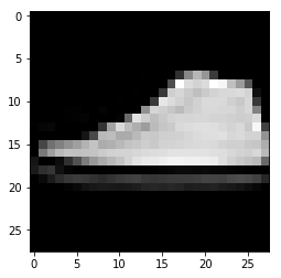
Let’s see what happens to image with the index 26 over all the layers of the CNN.
index = 41
This is the original image:
plt.imshow(x_train[index].reshape(28,28), cmap='gray');
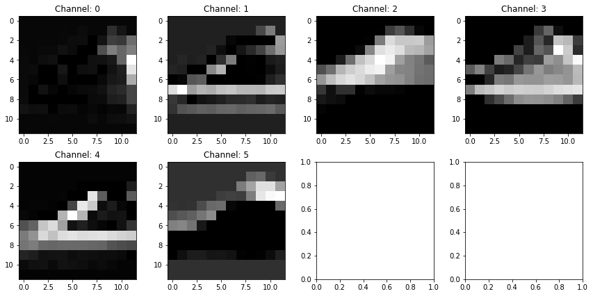
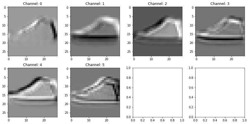
Output of convolution layer 1
Let’s take a look at the first convolution layer. For this layer:
- Input:
(None,32,32,1) - Filter size:
(5x5x1) - Num of filters:
6 - Strides:
(1,1) - Padding:
VALID
Output of this layer is of shape (None, 24, 24, 6)
fmnist_model.layers[1].output_shape
(None, 24, 24, 6)
conv1_layer_model = Model(inputs=fmnist_model.input,
                                 outputs=fmnist_model.layers[1].output)
conv1_output = conv1_layer_model.predict(x_train_scaled[index].reshape(1,28,28,1))
visualize_layer_output(conv1_output)
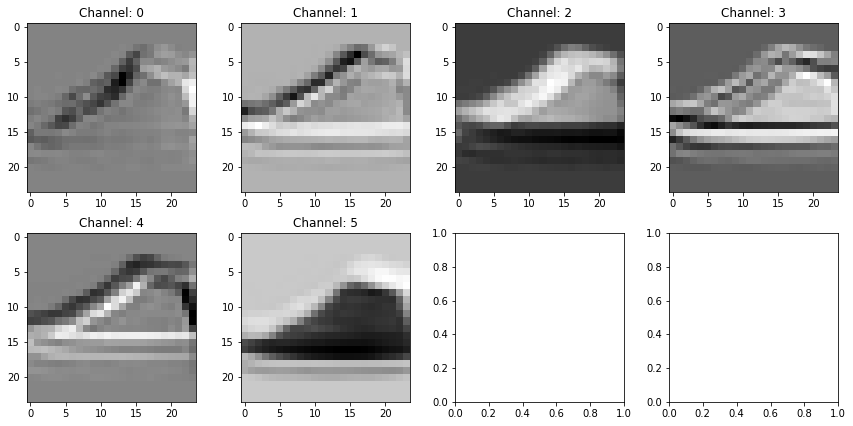
Each output (or channel) seems to be different from one another. For example, the sole of the sneaker is relatively differentiable from the rest of the shoe in channels 1,3, and 4, and much less in channels 0 and 5.
Output of first ReLU activation
act1_layer_model = Model(inputs=fmnist_model.input,
                                 outputs=fmnist_model.layers[2].output)
act1_output = act1_layer_model.predict(x_train_scaled[index].reshape(1,28,28,1))
visualize_layer_output(act1_output)
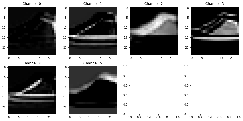
Again, the differentiablity of the sole of the sneaker is hightenend in channels 1,3, and 4.
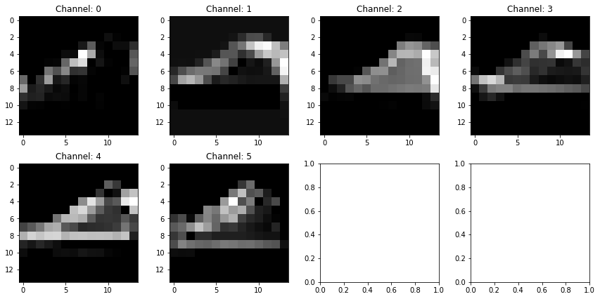
Output of Max Pool layer 1
Now to the first max pool layer. For this layer:
- Input:
(None, 24, 24, 6) - Pool size:
(2x2) - Strides:
(2,2) - Padding: VALID
Output of this layer is of shape (None, 12, 12, 6)
fmnist_model.layers[3].output_shape
(None, 12, 12, 6)
maxpool1_layer_model = Model(inputs=fmnist_model.input,
                                 outputs=fmnist_model.layers[3].output)
maxpool1_output = maxpool1_layer_model.predict(x_train_scaled[index].reshape(1,28,28,1))
visualize_layer_output(maxpool1_output)
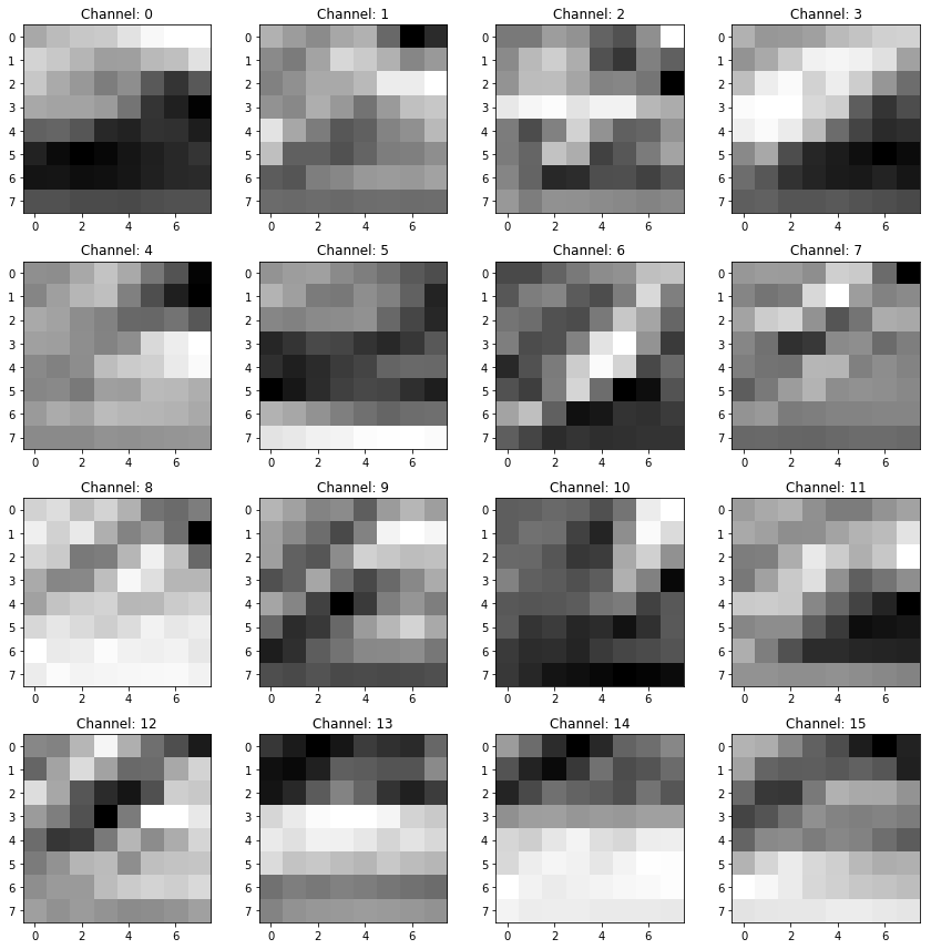
Output of Convolution layer 2
For the second convolution layer:
- Input:
(None, 12, 12, 6) - Filter size:
(5x5x1) - Num of filters:
16 - Strides:
(1,1) - Padding: VALID
Output of this layer is of shape (None, 8, 8, 16)
fmnist_model.layers[4].output_shape
(None, 8, 8, 16)
conv2_layer_model = Model(inputs=fmnist_model.input,
                                 outputs=fmnist_model.layers[4].output)
conv2_output = conv2_layer_model.predict(x_train_scaled[index].reshape(1,28,28,1))
visualize_layer_output(conv2_output)
Output of second ReLU activation
act2_layer_model = Model(inputs=fmnist_model.input,
                                 outputs=fmnist_model.layers[5].output)
act2_output = act2_layer_model.predict(x_train_scaled[index].reshape(1,28,28,1))
visualize_layer_output(act2_output)
Output of Max Pool layer 2
For the second max pool layer:
- Input:
(None, 8, 8, 16) - Pool size:
(2x2) - Strides:
(2,2) - Padding: VALID
Output of this layer is of shape (None, 4, 4, 16)
fmnist_model.layers[6].output_shape
(None, 4, 4, 16)
maxpool2_layer_model = Model(inputs=fmnist_model.input,
                                 outputs=fmnist_model.layers[6].output)
maxpool2_output = maxpool2_layer_model.predict(x_train_scaled[index].reshape(1,28,28,1))
visualize_layer_output(maxpool2_output)
Okay, I couldn’t make anything of the images after the first max-pool, probably because the resolution dropped too low after that. Just for visual perception, let’s write another variant of the model with ‘SAME’ padding in all of the layers.
def lenet5_variant_2(input_shape):

    X_input = Input(input_shape, name='input')

    X = Conv2D(6, (5, 5), strides = (1, 1), padding='same', name = 'conv1')(X_input)
    X = Activation('relu')(X)
    X = MaxPooling2D((2, 2), strides=(2,2), padding='same', name='max_pool1')(X)

    X = Conv2D(16, (5, 5), strides = (1, 1), padding='same', name = 'conv2')(X)
    X = Activation('relu')(X)
    X = MaxPooling2D((2, 2), strides=(2,2), padding='same', name='max_pool2')(X)

    X = Flatten()(X)
    X = Dense(120, activation='relu', name='fc1')(X)
    X = Dense(84, activation='relu', name='fc2')(X)
    X = Dense(10, activation='softmax', name='op')(X)

    model = Model(inputs = X_input, outputs = X, name='lenet5')
    return model
fmnist_model_2 = lenet5_variant_2((28,28,1))
fmnist_model_2.compile(optimizer=Adam(lr=0.001),
                   loss="categorical_crossentropy",
                   metrics=["accuracy"])
fmnist_model_2.fit(x = x_train_scaled, y = y_train, epochs = 30, batch_size = 64)
Epoch 1/30
60000/60000 [==============================] - 8s 129us/step - loss: 0.5263 - acc: 0.8090
Epoch 2/30
60000/60000 [==============================] - 7s 122us/step - loss: 0.3535 - acc: 0.8728
Epoch 3/30
60000/60000 [==============================] - 7s 120us/step - loss: 0.3027 - acc: 0.8902
Epoch 4/30
60000/60000 [==============================] - 7s 116us/step - loss: 0.2732 - acc: 0.8995
Epoch 5/30
60000/60000 [==============================] - 7s 114us/step - loss: 0.2495 - acc: 0.9075
Epoch 6/30
60000/60000 [==============================] - 7s 116us/step - loss: 0.2316 - acc: 0.9143
Epoch 7/30
60000/60000 [==============================] - 7s 115us/step - loss: 0.2164 - acc: 0.9186
Epoch 8/30
60000/60000 [==============================] - 7s 119us/step - loss: 0.1983 - acc: 0.9261
Epoch 9/30
60000/60000 [==============================] - 7s 116us/step - loss: 0.1870 - acc: 0.9296
Epoch 10/30
60000/60000 [==============================] - 7s 116us/step - loss: 0.1725 - acc: 0.9354
Epoch 11/30
60000/60000 [==============================] - 7s 115us/step - loss: 0.1594 - acc: 0.9399
Epoch 12/30
60000/60000 [==============================] - 7s 116us/step - loss: 0.1509 - acc: 0.9431
Epoch 13/30
60000/60000 [==============================] - 7s 118us/step - loss: 0.1409 - acc: 0.9459
Epoch 14/30
60000/60000 [==============================] - 7s 118us/step - loss: 0.1297 - acc: 0.9516
Epoch 15/30
60000/60000 [==============================] - 7s 115us/step - loss: 0.1218 - acc: 0.9542
Epoch 16/30
60000/60000 [==============================] - 7s 114us/step - loss: 0.1111 - acc: 0.9586
Epoch 17/30
60000/60000 [==============================] - 7s 116us/step - loss: 0.1028 - acc: 0.9615
Epoch 18/30
60000/60000 [==============================] - 7s 118us/step - loss: 0.0987 - acc: 0.9625
Epoch 19/30
60000/60000 [==============================] - 7s 114us/step - loss: 0.0874 - acc: 0.9679
Epoch 20/30
60000/60000 [==============================] - 7s 116us/step - loss: 0.0828 - acc: 0.9688
Epoch 21/30
60000/60000 [==============================] - 7s 116us/step - loss: 0.0769 - acc: 0.9710
Epoch 22/30
60000/60000 [==============================] - 7s 116us/step - loss: 0.0714 - acc: 0.9724
Epoch 23/30
60000/60000 [==============================] - 7s 115us/step - loss: 0.0655 - acc: 0.9751
Epoch 24/30
60000/60000 [==============================] - 7s 114us/step - loss: 0.0641 - acc: 0.9758
Epoch 25/30
60000/60000 [==============================] - 7s 116us/step - loss: 0.0602 - acc: 0.9774
Epoch 26/30
60000/60000 [==============================] - 7s 117us/step - loss: 0.0530 - acc: 0.9804
Epoch 27/30
60000/60000 [==============================] - 7s 117us/step - loss: 0.0516 - acc: 0.9812
Epoch 28/30
60000/60000 [==============================] - 7s 116us/step - loss: 0.0510 - acc: 0.9810
Epoch 29/30
60000/60000 [==============================] - 7s 116us/step - loss: 0.0447 - acc: 0.9832
Epoch 30/30
60000/60000 [==============================] - 7s 115us/step - loss: 0.0450 - acc: 0.9841
<keras.callbacks.History at 0x7fb82eddcbe0>
Conv-1
conv1_layer_model_2 = Model(inputs=fmnist_model_2.input,
                                 outputs=fmnist_model_2.layers[1].output)
conv1_output_2 = conv1_layer_model_2.predict(x_train_scaled[index].reshape(1,28,28,1))
visualize_layer_output(conv1_output_2)
Max-pool-1
maxpool1_layer_model_2 = Model(inputs=fmnist_model_2.input,
                                 outputs=fmnist_model_2.layers[3].output)
maxpool1_output_2 = maxpool1_layer_model_2.predict(x_train_scaled[index].reshape(1,28,28,1))
visualize_layer_output(maxpool1_output_2)
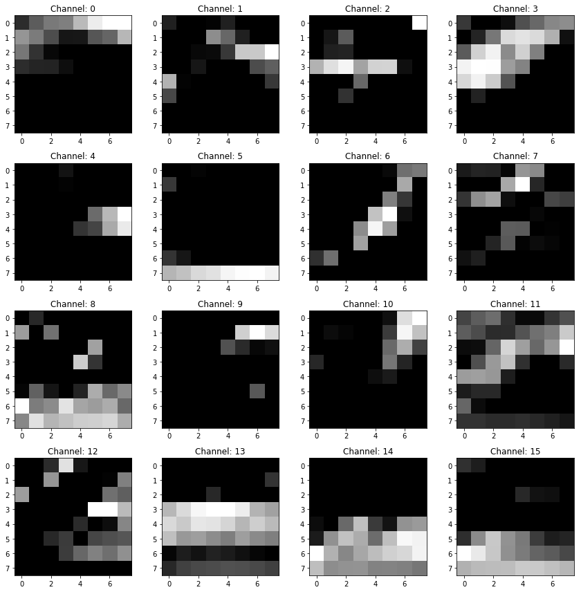
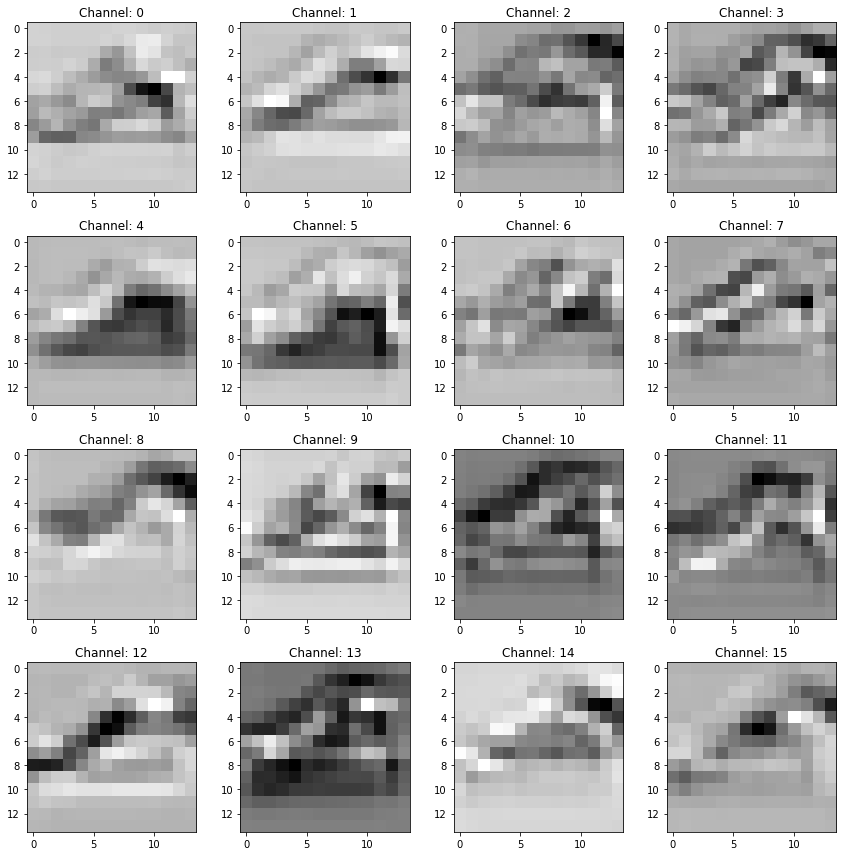
Conv-2
conv2_layer_model_2 = Model(inputs=fmnist_model_2.input,
                                 outputs=fmnist_model_2.layers[4].output)
conv2_output_2 = conv2_layer_model_2.predict(x_train_scaled[index].reshape(1,28,28,1))
visualize_layer_output(conv2_output_2)
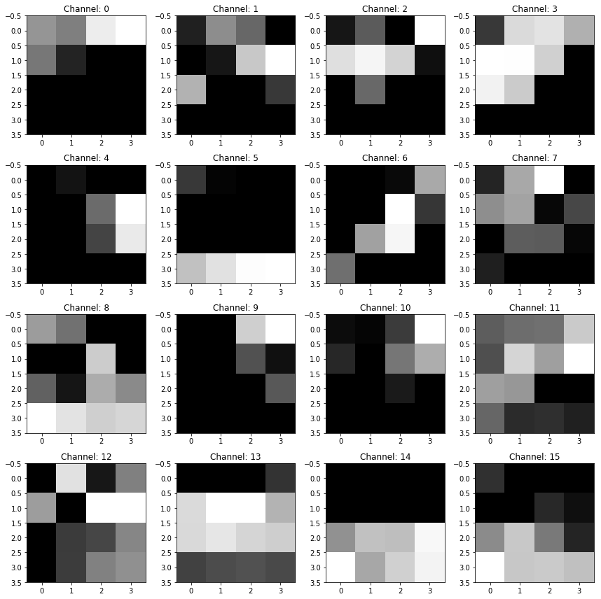
Max-pool-2
maxpool2_layer_model_2 = Model(inputs=fmnist_model_2.input,
                                 outputs=fmnist_model_2.layers[6].output)
maxpool2_output_2 = maxpool2_layer_model_2.predict(x_train_scaled[index].reshape(1,28,28,1))
visualize_layer_output(maxpool2_output_2)
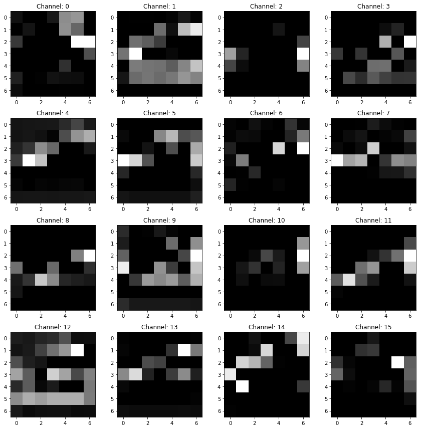
In summary, as seen above, different channels in a CNN layer propagate different representations of it’s input. Next, I’ll try to do the same with larger images and some other CNN architecture.