The first and second courses by deeplearning.ai offer a great insight into the working of various optimisation algorithms used in Machine Learning. Specifically, they focus on Batch Gradient Descent, Mini-batch Gradient Descent (with and without momentum), and Adam optimisation. Having finished the two courses, I’ve wanted to go deeper into the world of optimisation. This is probably the first step towards that.
This notebook/post is an introductory level analysis on the workings of these optimisation approaches. The intent is to visually see these algorithms in action, and hopefully see how they’re different from each other.
The approach below is greatly inspired by this post by Louis Tiao on optimisation visualizations, and this tutorial on matplotlib animation by Jake VanderPlas.
Setup
# imports
import matplotlib.pyplot as plt
import numpy as np
from mpl_toolkits.mplot3d import Axes3D
from matplotlib.colors import LogNorm
from matplotlib import animation
from IPython.display import HTML
import math
from itertools import zip_longest
from sklearn.datasets import make_classification
%matplotlib inline
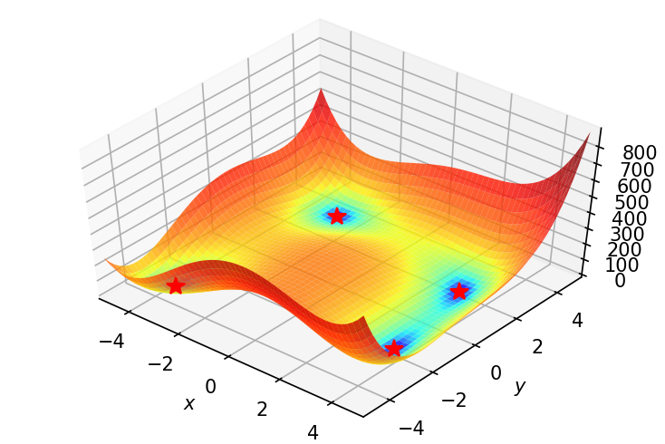
Alright. We need something to optimize. To begin with, let’s try to find the minima(s) of Himmelblau function , which is represented as:
$$\large f(x,y)=(x^{2}+y-11)^{2}+(x+y^{2}-7)^{2}$$
This function as 4 minimas:
- $f(3.0,2.0)=0.0$
- $f(-2.805118,3.131312)=0.0$
- $f(-3.779310,-3.283186)=0.0$
- $f(3.584428,-1.848126)=0.0$
Writing the function in Python:
f = lambda x, y: (x**2 +y -11)**2 + (x + y**2 -7)**2
xmin, xmax, xstep = -5, 5, .2
ymin, ymax, ystep = -5, 5, .2
Let’s see a 3d plot of the function. Creating a meshgrid so as to plot contours:
x, y = np.meshgrid(np.arange(xmin, xmax + xstep, xstep), np.arange(ymin, ymax + ystep, ystep))
z = f(x, y)
Creating 4 minima variables to display on the plot.
minima1 = np.array([3., 2.])
minima2 = np.array([-2.80, 3.13])
minima3 = np.array([-3.78, -3.3])
minima4 = np.array([3.6, -1.85])

minima1_ = minima1.reshape(-1, 1)
minima2_ = minima2.reshape(-1, 1)
minima3_ = minima3.reshape(-1, 1)
minima4_ = minima4.reshape(-1, 1)
Plotting.
fig = plt.figure(dpi=150, figsize=(6, 4))
ax = plt.axes(projection='3d', elev=50, azim=-50)

ax.plot_surface(x, y, z, norm=LogNorm(), rstride=1, cstride=1,
                edgecolor='none', alpha=.8, cmap=plt.cm.jet)
ax.plot(*minima1_, f(*minima1_), 'r*', markersize=10)
ax.plot(*minima2_, f(*minima2_), 'r*', markersize=10)
ax.plot(*minima3_, f(*minima3_), 'r*', markersize=10)
ax.plot(*minima4_, f(*minima4_), 'r*', markersize=10)

ax.set_xlabel('$x$')
ax.set_ylabel('$y$')
ax.set_zlabel('$z$')

ax.set_xlim((xmin, xmax))
ax.set_ylim((ymin, ymax))

plt.show()
We need gradients of the function f wrt x and y to code the optimisation logic.
dx = lambda x, y: 2*(x**2 +y -11)*2*x + 2*(x + y**2 -7)
dy = lambda x, y: 2*(x**2 +y -11) + 2*(x + y**2 -7)*2*y
Writing a simple implementation of gradient descent. Also keeping a track of the values of x and y in the path variable while the algorithms descends to the minima. GD will run for num_epochs iterations.
def gradient_descent(init_point,learning_rate, num_epochs):
    x0 = init_point[0]
    y0 = init_point[1]

    path = np.zeros((2,num_epochs+1))

    path[0][0] = x0
    path[1][0] = y0

    for i in range(num_epochs):
        x_ =  learning_rate*dx(x0,y0)
        y_ =  learning_rate*dy(x0,y0)
        x0 -= x_
        y0 -= y_
        path[0][i+1] = x0
        path[1][i+1] = y0

    return (path,(x0,y0))
Choosing a few starting points. We’ll initialize GD separately with all of these and plot the paths taken in each case.
begin_points = [
    np.array([0.,0.]),
    np.array([-0.5,0.]),
    np.array([-0.5,-0.5]),
    np.array([0.5,-0.5]),
    np.array([0.5,-0.5]),
    np.array([-1.23633,-1.11064]),
    np.array([0.295466,-1.2946]),
    np.array([0.3616,4.9298]),
    np.array([1.362,-4.774]),
               ]
All paths will be stored in the paths variable. In order to make the plot clean, selecting a subset of the each path (every 5th point).
paths = []
for begin_point in begin_points:
    path,_ = gradient_descent(begin_point,learning_rate=0.001, num_epochs=300)
    path = path[:, [i for i in range(0,path.shape[1],5)]]
    paths.append(path)
Gradient descent is complete for all the starting points. Let’s see the paths taken on a contour plot of the function.
fig, ax = plt.subplots(dpi=150, figsize=(8, 6))

ax.contour(x, y, z, levels=np.logspace(0, 5, 35), norm=LogNorm(), cmap=plt.cm.jet)

for i,path in enumerate(paths):
    color = c=np.random.rand(3,)
    ax.quiver(path[0,:-1], path[1,:-1], path[0,1:]-path[0,:-1], path[1,1:]-path[1,:-1],\
              scale_units='xy', angles='xy', scale=1, color=color)
    ax.plot(*begin_points[i], color=color ,marker='o', markersize=10)

ax.plot(*minima1_, 'r*', markersize=18)
ax.plot(*minima2_, 'r*', markersize=18)
ax.plot(*minima3_, 'r*', markersize=18)
ax.plot(*minima4_, 'r*', markersize=18)

ax.set_xlabel('$x$')
ax.set_ylabel('$y$')

ax.set_xlim((xmin, xmax))
ax.set_ylim((ymin, ymax))

plt.show()
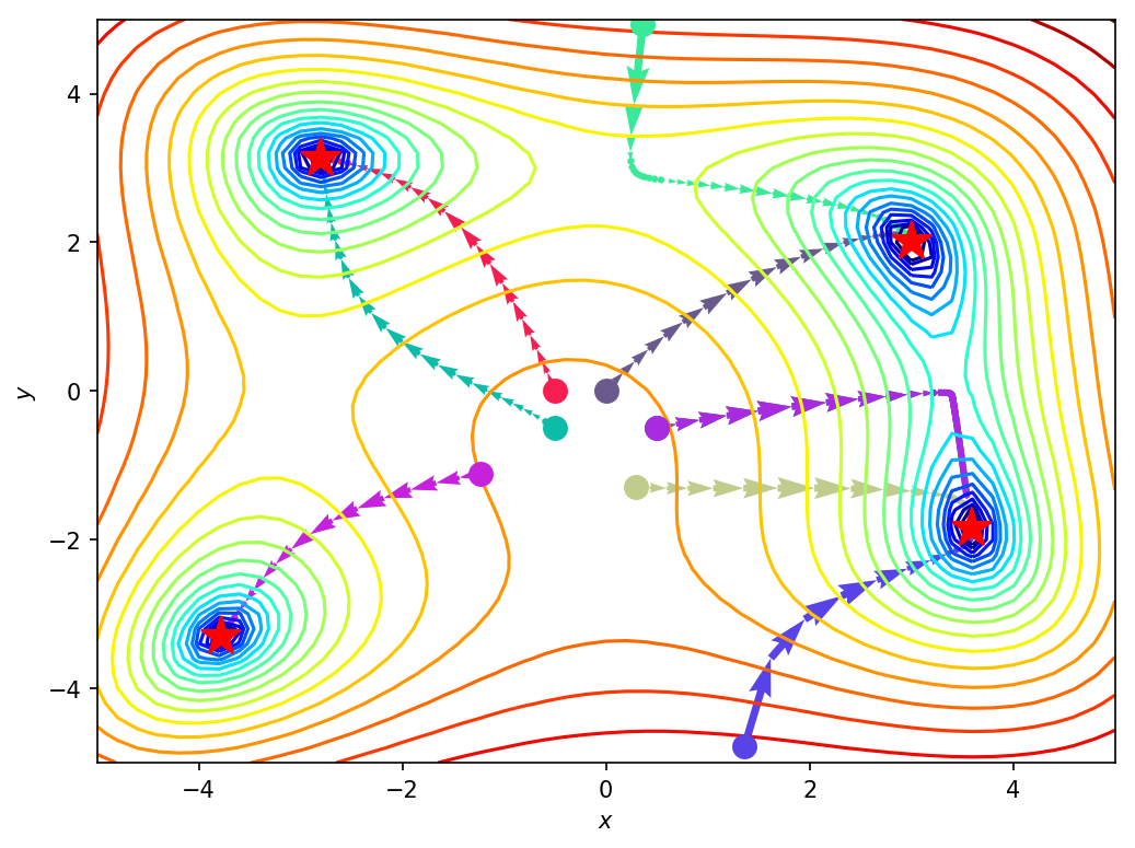
Nice! As seen above, starting point greatly influences where the algorithm converges.
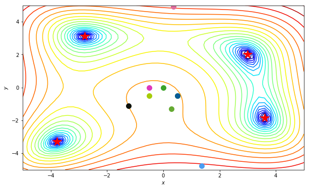
Time to see it in animation. Making use of the following class written by Louis to generate matplotlib animations for multiple paths:
class TrajectoryAnimation(animation.FuncAnimation):

    def __init__(self, *paths, labels=[], fig=None, ax=None, frames=None,
                 interval=60, repeat_delay=5, blit=True, **kwargs):

        if fig is None:
            if ax is None:
                fig, ax = plt.subplots()
            else:
                fig = ax.get_figure()
        else:
            if ax is None:
                ax = fig.gca()

        self.fig = fig
        self.ax = ax

        self.paths = paths

        if frames is None:
            frames = max(path.shape[1] for path in paths)

        self.lines = [ax.plot([], [], label=label, lw=2)[0]
                      for _, label in zip_longest(paths, labels)]
        self.points = [ax.plot([], [], 'o', color=line.get_color())[0]
                       for line in self.lines]

        super(TrajectoryAnimation, self).__init__(fig, self.animate, init_func=self.init_anim,
                                                  frames=frames, interval=interval, blit=blit,
                                                  repeat_delay=repeat_delay, **kwargs)

    def init_anim(self):
        for line, point in zip(self.lines, self.points):
            line.set_data([], [])
            point.set_data([], [])
        return self.lines + self.points

    def animate(self, i):
        for line, point, path in zip(self.lines, self.points, self.paths):
            line.set_data(*path[::,:i])
            point.set_data(*path[::,i-1:i])
        return self.lines + self.points
fig, ax = plt.subplots(figsize=(10, 6))

ax.contour(x, y, z, levels=np.logspace(0, 5, 35), norm=LogNorm(), cmap=plt.cm.jet)

for i,path in enumerate(paths):
    color = c=np.random.rand(3,)
    ax.plot(*begin_points[i].reshape(-1,1), color=color ,marker='o', markersize=10)

ax.plot(*minima1_, 'r*', markersize=18)
ax.plot(*minima2_, 'r*', markersize=18)
ax.plot(*minima3_, 'r*', markersize=18)
ax.plot(*minima4_, 'r*', markersize=18)

ax.set_xlabel('$x$')
ax.set_ylabel('$y$')

ax.set_xlim((xmin, xmax))
ax.set_ylim((ymin, ymax))

anim = TrajectoryAnimation(*paths, ax=ax)

# ax.legend(loc='upper left')
HTML(anim.to_html5_video())
Sweet! Let’s move on to a more concrete example.
np.random.seed(1)
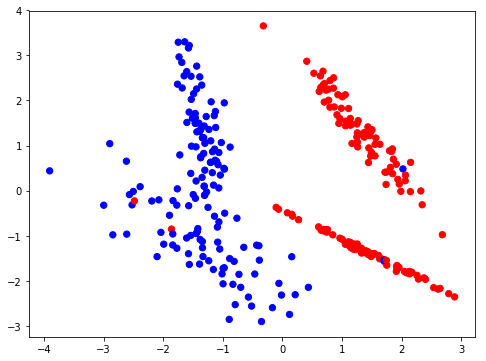
Creating a simple classification dataset for logistic regression.
X,Y = make_classification(n_samples=300, n_features=2, n_classes=2,n_redundant=0,class_sep=1.3)

X = X.T
Y = Y.T.reshape(1,-1)

plt.figure(figsize=(8,6))
plt.scatter(X[0, :], X[1, :], c=Y[0,:], s=40, cmap=plt.cm.bwr);
I’m going to implement logistic regression with the mindset of a simple neural network, ie, a single neuron in the only layer of the network (output layer). Writing down the functions to implement the network.
First a simple sigmoid function.
def sigmoid(x):
    s = 1/(1+np.exp(-x))
    return s
layer_sizes simply returns the number of inputs and outputs (2 and 1 in this case).
def layer_sizes(X, Y):
    n_x = X.shape[0]
    n_y = Y.shape[0]
    return (n_x, n_y)
Initializing the weights (having shape (1,2)) with random numbers, and the bias (having shape (1,1)) with zeros.
def initialize_parameters(n_x, n_y):
    np.random.seed(2)
    W1 = np.random.randn(n_y,n_x)*0.01
    b1 = np.random.randn(n_y,1)*0.01
    parameters = {"W1": W1,
                  "b1": b1}

    return parameters
Code for forward propagation. Returns the sigmoid activation of the linear activation of the neuron. Also returns a cache of the linear and sigmoid activations to be used later for back propagation. I’ve written more about this approach of forward and back-prop here.
def forward_propagation(X, parameters):
    W1 = parameters["W1"]
    b1 = parameters["b1"]

    Z1 = np.matmul(W1,X) + b1
    A1 = sigmoid(Z1)
    cache = {"Z1": Z1,
             "A1": A1}

    return A1, cache
Cost computation.
def compute_cost(A1, Y, parameters):
    m = Y.shape[1]
    logprobs = None
    cost = (-1/m)*(np.matmul(Y,np.log(A1).T) + np.matmul(1-Y,np.log(1-A1).T))
    cost = float(np.squeeze(cost))

    return cost
Calculates and returns gradients of the weights and biases wrt to the cost. Uses cache generated during forward propagation for simplifying calculation.
def backward_propagation(parameters, cache, X, Y):
    m = X.shape[1]
    W1 = parameters["W1"]
    A1 = cache["A1"]
    dZ1 = A1 - Y
    dW1 = (1/m)*np.matmul(dZ1,X.T)
    db1 = (1/m)*np.sum(dZ1, axis=1,keepdims=True)

    grads = {"dW1": dW1,
             "db1": db1}

    return grads
Updating parameters as per gradient descent.
def update_parameters(parameters, grads, learning_rate):
    W1 = parameters["W1"]
    b1 = parameters["b1"]

    dW1 = grads["dW1"]
    db1 = grads["db1"]

    W1 = W1 - learning_rate*dW1
    b1 = b1 - learning_rate*db1

    parameters = {"W1": W1,
                  "b1": b1}

    return parameters
learn_and_return_costs_batch_gd trains the neuron, and also returns the history of weights and costs. This is similar to the how we used the variable path above.
def learn_and_return_costs_batch_gd(X, Y, w, learning_rate, num_epochs):

    np.random.seed(3)
    n_x = layer_sizes(X, Y)[0]
    n_y = layer_sizes(X, Y)[1]

    parameters = initialize_parameters(n_x, n_y)
    W1 = parameters["W1"]
    b1 = parameters["b1"]
    parameters["W1"][0][0] = w[0]
    parameters["W1"][0][1] = w[1]

    wts1 = []
    wts2 = []
    costs = []
    params = []

    for i in range(0, num_epochs):
        A1, cache = forward_propagation(X, parameters)

        cost = compute_cost(A1, Y, parameters)

        grads = backward_propagation(parameters, cache, X, Y)

        if i % 800 == 0:
            wts1.append(parameters["W1"][0][0])
            wts2.append(parameters["W1"][0][1])
            costs.append(cost)
        if i % 5000 == 0:
            params.append(parameters)

        parameters = update_parameters(parameters, grads, learning_rate = learning_rate)

    return wts1,wts2,costs,params
To generate contour plots of cost wrt to the two weights we need calc_cost_for_weights which simply performs forward propagation and calculates the cost.
def calc_cost_for_weights(X, Y, w):

    np.random.seed(3)
    n_x = layer_sizes(X, Y)[0]
    n_y = layer_sizes(X, Y)[1]

    parameters = initialize_parameters(n_x, n_y)
    parameters["W1"][0][0] = w[0]
    parameters["W1"][0][1] = w[1]
    W1 = parameters["W1"]
    b1 = parameters["b1"]

    A1, cache = forward_propagation(X, parameters)

    cost = compute_cost(A1, Y, parameters)

    return cost
Let’s start with a range of weights distributed between (-4,4).
W = np.array([np.linspace(-4,4, num=100), np.linspace(-4,4, num=100)]).T
W.shape
(100, 2)
(W[0][0],W[0][1])
(-4.0, -4.0)
Training the neuron with the weights initialized to (-4.0, -4.0). Running gradient descent for $3000$ epochs with a learning rate of $0.001$.
wts1,wts2,costs,params_learnt = learn_and_return_costs_batch_gd(X,Y,(W[0][0],W[0][1]),\
                                                                learning_rate=0.001,\
                                                                num_epochs=3000)
Okay. The neuron is trained. Time to plot the path taken by gradient descent. For that we need first generate a contour plot of the cost wrt to the two weights.
squared_error_vals = np.zeros(shape=(W[:, 0].size, W[:, 1].size))
for i, w1 in enumerate(W[:, 0]):
    for j, w2 in enumerate(W[:, 1]):
        w = np.array([w1, w2])
        squared_error = calc_cost_for_weights(X,Y,w)
        squared_error_vals[i, j] = squared_error
squared_error_vals.shape
(100, 100)
Batch Gradient Descent
Plotting the path taken on a contour plot.
fig = plt.figure(dpi=150, figsize=(5,5))
cp = plt.contour(W[:,0], W[:, 1], squared_error_vals, np.logspace(-6, 6, 30), cmap=plt.cm.bwr)
plt.clabel(cp, inline=1, fontsize=8)
min_point = np.unravel_index(squared_error_vals.argmin(), squared_error_vals.shape)

plt.plot(W[min_point[1],1],W[min_point[0],0], 'g*', markersize=10)
plt.plot(wts2[0],wts1[0], 'ro')

for i in range(1, len(wts1)):
    plt.plot(wts2[i],wts1[i], 'bo', markersize=3)
    plt.annotate('', xy=(wts2[i], wts1[i]), xytext=(wts2[i-1], wts1[i-1]),
                   arrowprops={'arrowstyle': '->', 'color': 'r', 'lw': 1},
                   va='center', ha='center')
plt.tight_layout()

print('Starting cost weights grid: {:0.3f}'.format(costs[0]))
print('Min cost on weights grid: {:0.3f}'.format(np.amin(squared_error_vals)))

plt.show()
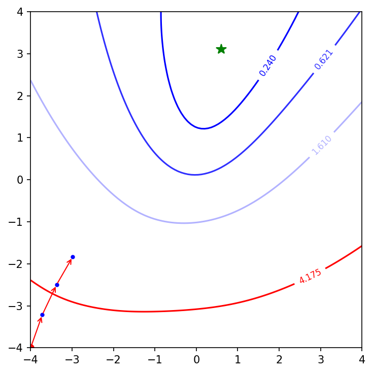
The green star is the minima of the cost function for this range of weights. The implementation of learn_and_return_costs_batch_gd is only storing the values of weights every $800$ epoch. So the plot only contains 3 points in the journey of gradient descent. Lets increase the number of epochs to $6000$ and plot again.
wts1,wts2,costs,params_learnt = learn_and_return_costs_batch_gd(X,Y,(W[0][0],W[0][1]),\
                                                                learning_rate=0.001,\
                                                                num_epochs=6000)

squared_error_vals = np.zeros(shape=(W[:, 0].size, W[:, 1].size))
for i, w1 in enumerate(W[:, 0]):
    for j, w2 in enumerate(W[:, 1]):
        w = np.array([w1, w2])
        squared_error = calc_cost_for_weights(X,Y,w)
        squared_error_vals[i, j] = squared_error

fig = plt.figure(dpi=150, figsize=(5,5))
cp = plt.contour(W[:,0], W[:, 1], squared_error_vals, np.logspace(-6, 6, 30), cmap=plt.cm.bwr)
plt.clabel(cp, inline=1, fontsize=8)
min_point = np.unravel_index(squared_error_vals.argmin(), squared_error_vals.shape)

plt.plot(W[min_point[1],1],W[min_point[0],0], 'g*', markersize=10)
plt.plot(wts2[0],wts1[0], 'ro')

for i in range(1, len(wts1)):
    plt.plot(wts2[i],wts1[i], 'bo', markersize=3)
    plt.annotate('', xy=(wts2[i], wts1[i]), xytext=(wts2[i-1], wts1[i-1]),
                   arrowprops={'arrowstyle': '->', 'color': 'r', 'lw': 1},
                   va='center', ha='center')
plt.tight_layout()

print('Starting cost weights grid: {:0.3f}'.format(costs[0]))
print('Min cost on weights grid: {:0.3f}'.format(np.amin(squared_error_vals)))

plt.show()
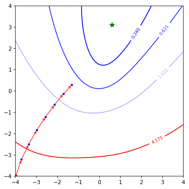
Okay, now we see more steps taken by GD. I want to compare performance of batch GD with other optimisation algorithms. Let’s compare it with mini-batch gradient descent, mini-batch gradient descent with momentum, and mini-batch adam optimisation.
Function to generate random mini batches of the entire dataset. Setting default mini-batch size to 64.
def random_mini_batches(X, Y, mini_batch_size = 64, seed = 0):

    np.random.seed(seed)
    m = X.shape[1]
    mini_batches = []

    permutation = list(np.random.permutation(m))
    shuffled_X = X[:, permutation]
    shuffled_Y = Y[:, permutation].reshape((1,m))

    num_complete_minibatches = math.floor(m/mini_batch_size)
    for k in range(0, num_complete_minibatches):
        mini_batch_X = shuffled_X[:,(k)*mini_batch_size:(k+1)*mini_batch_size]
        mini_batch_Y = shuffled_Y[:,(k)*mini_batch_size:(k+1)*mini_batch_size]
        mini_batch = (mini_batch_X, mini_batch_Y)
        mini_batches.append(mini_batch)

    if m % mini_batch_size != 0:
        mini_batch_X = shuffled_X[:,(num_complete_minibatches)*mini_batch_size:]
        mini_batch_Y = shuffled_Y[:,(num_complete_minibatches)*mini_batch_size:]
        mini_batch = (mini_batch_X, mini_batch_Y)
        mini_batches.append(mini_batch)

    return mini_batches
Initializing velocity with zeros for mini-batch GD with momentum.
def initialize_velocity(parameters):
    L = len(parameters) // 2
    v = {}

    for l in range(L):
        v["dW" + str(l+1)] = np.zeros((parameters["W" + str(l+1)].shape[0],parameters["W" + str(l+1)].shape[1]))
        v["db" + str(l+1)] = np.zeros((parameters["b" + str(l+1)].shape[0],parameters["b" + str(l+1)].shape[1]))

    return v
Update rule for mini-batch GD with momentum:
$$ \large v_{dW} = \beta v_{dW} + (1 - \beta) dW $$
$$ \large W = W - \alpha v_{dW} $$
$$ \large v_{db} = \beta v_{db} + (1 - \beta) db $$
$$ \large b = b - \alpha v_{db} $$
where $\beta$ is the momentum and $\alpha$ is the learning rate.
def update_parameters_with_momentum(parameters, grads, v, beta, learning_rate):
    L = len(parameters) // 2

    for l in range(L):

        v["dW" + str(l+1)] = beta*v["dW" + str(l+1)] + (1-beta)*grads["dW"+str(l+1)]
        v["db" + str(l+1)] = beta*v["db" + str(l+1)] + (1-beta)*grads["db"+str(l+1)]
        parameters["W" + str(l+1)] -= learning_rate*v["dW" + str(l+1)]
        parameters["b" + str(l+1)] -= learning_rate*v["db" + str(l+1)]

    return parameters, v
Now let’s code up the helper functions for Adam. In this implementation of Adam v[parameter] represents biased first moment estimate, s[parameter] represents biased second raw moment estimate.
def initialize_adam(parameters) :
    L = len(parameters)//2
    v = {}
    s = {}

    for l in range(L):
        v["dW" + str(l+1)] = np.zeros((parameters["W" + str(l+1)].shape[0],parameters["W" + str(l+1)].shape[1]))
        v["db" + str(l+1)] = np.zeros((parameters["b" + str(l+1)].shape[0],parameters["b" + str(l+1)].shape[1]))
        s["dW" + str(l+1)] = np.zeros((parameters["W" + str(l+1)].shape[0],parameters["W" + str(l+1)].shape[1]))
        s["db" + str(l+1)] = np.zeros((parameters["b" + str(l+1)].shape[0],parameters["b" + str(l+1)].shape[1]))
    return v, s
Function to update adam specific parameters. beta1, beta2, and epsilon all default to the values suggested by the original paper.
Update logic:
$$ \large v_{W} = \beta_1 v_{W} + (1 - \beta_1) \frac{\partial J }{ \partial W } $$
$$ \large v^{corrected}{W} = \frac{v{W}}{1 - (\beta_1)^t} $$
$$ \large s_{W} = \beta_2 s_{W} + (1 - \beta_2) (\frac{\partial J }{\partial W })^2$$
$$ \large s^{corrected}{W} = \frac{s{W}}{1 - (\beta_2)^t}$$
$$ \large W = W - \alpha \frac{v^{corrected}{W}}{\sqrt{s^{corrected}{W}}+\varepsilon}$$
def update_parameters_with_adam(parameters, grads, v, s, t, learning_rate = 0.01,
                                beta1 = 0.9, beta2 = 0.999,  epsilon = 1e-8):
    L = len(parameters) // 2
    v_corrected = {}
    s_corrected = {}

    for l in range(L):
        v["dW" + str(l+1)] = beta1*v["dW" + str(l+1)] + (1-beta1)*grads["dW" + str(l+1)]
        v["db" + str(l+1)] = beta1*v["db" + str(l+1)] + (1-beta1)*grads["db" + str(l+1)]

        v_corrected["dW" + str(l+1)] = v["dW" + str(l+1)]/(1-math.pow(beta1,t))
        v_corrected["db" + str(l+1)] = v["db" + str(l+1)]/(1-math.pow(beta1,t))

        s["dW" + str(l+1)] = beta2*s["dW" + str(l+1)] + (1-beta2)*np.square(grads["dW" + str(l+1)])
        s["db" + str(l+1)] = beta2*s["db" + str(l+1)] + (1-beta2)*np.square(grads["db" + str(l+1)])

        s_corrected["dW" + str(l+1)] = s["dW" + str(l+1)]/(1-math.pow(beta2,t))
        s_corrected["db" + str(l+1)] = s["db" + str(l+1)]/(1-math.pow(beta2,t))

        parameters["W" + str(l+1)] -= learning_rate*(v_corrected["dW" + str(l+1)]/(np.sqrt(s_corrected["dW" + str(l+1)])+epsilon))
        parameters["b" + str(l+1)] -= learning_rate*(v_corrected["db" + str(l+1)]/(np.sqrt(s_corrected["db" + str(l+1)])+epsilon))

    return parameters, v, s
Generic implementation of training for mini-batch GD, mini-batch GD with momentum, and mini-batch Adam. Just like learn_and_return_costs_batch_gd it returns history of weights saved at every $800$th epoch for comparison metrics.
def learn_and_return_costs_mini_batch(X, Y, w, optimizer, learning_rate, num_epochs, mini_batch_size = 64, beta = 0.9,
          beta1 = 0.9, beta2 = 0.999,  epsilon = 1e-8, print_cost = True):
    costs = []
    t = 0
    seed = 10
    n_x = layer_sizes(X, Y)[0]
    n_y = layer_sizes(X, Y)[1]

    parameters = initialize_parameters(n_x, n_y)
    W1 = parameters["W1"]
    b1 = parameters["b1"]
    parameters["W1"][0][0] = w[0]
    parameters["W1"][0][1] = w[1]

    wts1 = []
    wts2 = []
    costs = []
    params = []

    counter = 0

    costs_for_graph = []

    if optimizer == "gd":
        pass
    elif optimizer == "momentum":
        v = initialize_velocity(parameters)
    elif optimizer == "adam":
        v, s = initialize_adam(parameters)

    for i in range(num_epochs):

        seed = seed + 1
        minibatches = random_mini_batches(X, Y, mini_batch_size, seed)

        for minibatch in minibatches:

            (minibatch_X, minibatch_Y) = minibatch

            a1, caches = forward_propagation(minibatch_X, parameters)

            cost = compute_cost(a1, minibatch_Y, parameters)

            grads = backward_propagation(parameters,caches,minibatch_X, minibatch_Y,)

            if counter % 800 == 0:
                wts1.append(parameters["W1"][0][0])
                wts2.append(parameters["W1"][0][1])
                costs.append(cost)
            if counter % 5000 == 0:
                params.append(parameters)

            parameters = update_parameters(parameters, grads, learning_rate = learning_rate)
            counter+=1

            if optimizer == "gd":
                parameters = update_parameters(parameters, grads, learning_rate)
            elif optimizer == "momentum":
                parameters, v = update_parameters_with_momentum(parameters, grads, v, beta, learning_rate)
            elif optimizer == "adam":
                t = t + 1
                parameters, v, s = update_parameters_with_adam(parameters, grads, v, s,
                                                               t, learning_rate, beta1, beta2,  epsilon)

    return wts1,wts2,costs,params
Okay. Time for plotting. I’ve wrapped the plotting code in a generic function for various optimisation algorithm choices.
def plot_optimisation(optimizer, learning_rate, num_epochs):
    layers_dims = [X.shape[0], 1]
    W = np.array([np.linspace(-4,4, num=100), np.linspace(-4,4, num=100)]).T

    wts1,wts2,costs,params_learnt = learn_and_return_costs_mini_batch(X,Y,(W[0][0],W[0][1]), optimizer,\
                                                                      learning_rate,\
                                                                      num_epochs,\
                                                                      print_cost=False)

    squared_error_vals = np.zeros(shape=(W[:, 0].size, W[:, 1].size))
    for i, w1 in enumerate(W[:, 0]):
        for j, w2 in enumerate(W[:, 1]):
            w = np.array([w1, w2])
            squared_error = calc_cost_for_weights(X,Y,w)
            squared_error_vals[i, j] = squared_error

    fig = plt.figure(dpi=150, figsize=(5,5))
    cp = plt.contour(W[:,0], W[:, 1], squared_error_vals, np.logspace(-6, 6, 30), cmap=plt.cm.bwr)
    plt.clabel(cp, inline=1, fontsize=8)
    min_point = np.unravel_index(squared_error_vals.argmin(), squared_error_vals.shape)
    plt.plot(W[min_point[1],1],W[min_point[0],0], 'g*', markersize=10)

    plt.plot(wts2[0],wts1[0], 'ro')

    for i in range(1, len(wts1)):
        plt.plot(wts2[i],wts1[i], 'bo', markersize=3)
        plt.annotate('', xy=(wts2[i], wts1[i]), xytext=(wts2[i-1], wts1[i-1]),
                       arrowprops={'arrowstyle': '->', 'color': 'r', 'lw': 1},
                       va='center', ha='center')
    print('Starting cost weights grid: {:0.3f}'.format(costs[0]))
    print('Min cost on weights grid: {:0.3f}'.format(np.amin(squared_error_vals)))

#     plt.tight_layout()
    plt.show()
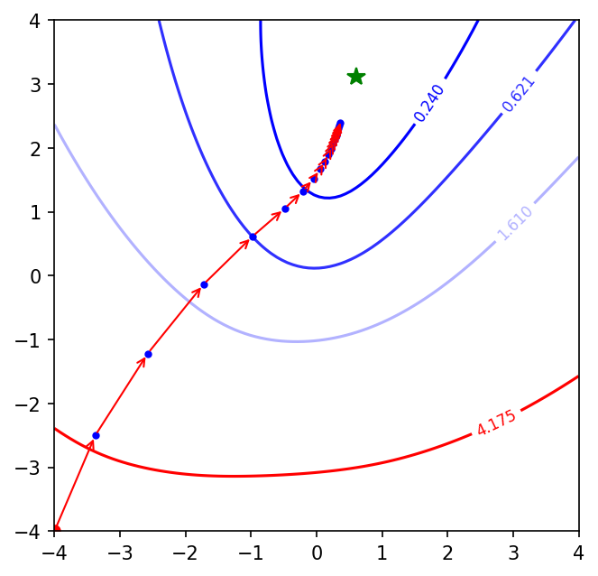
Mini-Batch Gradient Descent
Let’s run mini-batch GD for 3000 epochs like we did for batch GD.
plot_optimisation(optimizer='gd', learning_rate=0.001, num_epochs=3000)

Okay! Mini-batch GD makes more progress than batch GD for the same number of epochs. It is almost near the minima. Let’s run it with mini-batch GD with momentum.
Mini-Batch Gradient Descent with Momentum
plot_optimisation(optimizer='momentum', learning_rate=0.001, num_epochs=3000)
Similar performance like mini-batch GD. Let’s run it for Adam.
Adam optimisation
plot_optimisation(optimizer='adam', learning_rate=0.001, num_epochs=3000)
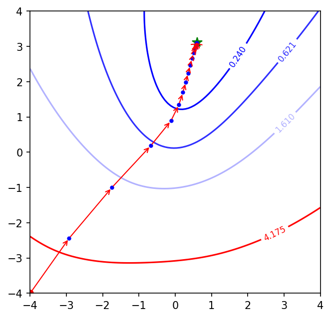
Adam has converged within 3000 epochs. From the above plots we can see that mini-batch GD (with and without momentum) and Adam speed up the convergence process a lot more than batch GD. Also, Adam takes the most efficient steps towards the minimum amongst the three as evident from the blue points which represent every 800th epoch. The length of the arrows between 2 blue points is the largest in Adam’s case.
This was a fun exercise for me. I’ll probably do something like this again once I learn about other optimisation algorithms. Hopefully by then, I’ll be able to create even more slick matplotlib animations.